Introduction
The Atlantic sea scallop (Placopecten magellanicus) fishery is the most valuable single-species fishery along the eastern coast of the United States (US; van Voorhees, MS 2014). The species is distributed along the northeastern US continental shelf from Cape Hatteras, North Carolina, to Maine, but the bulk of the fishery’s effort is concentrated on the productive scallop beds in the mid-Atlantic Bight and on Georges Bank (NEFMC, MS 2014). Since 2004, the resource has been harvested under a rotational area-based management strategy designed to increase the long-term yield and reproductive potential of the stock by identifying and protecting high-density beds of juvenile scallops from fishing mortality (NEFMC, MS 2003). Under the current plan, the fleet is also given limited access to two static closed areas on Georges Bank (Closed Areas I and II, hereafter also referred to as scallop access areas; Fig. 1) that were established in 1994 to protect spawning habitat of depleted groundfish stocks (Murawski et al., 2000). Although this management strategy has resulted in increased scallop yields (NEFSC, MS 2010), bycatch of several groundfish species remains a constraint to the fishery, both on Georges Bank and in the mid-Atlantic (O’Keefe and DeCelles, 2013).
 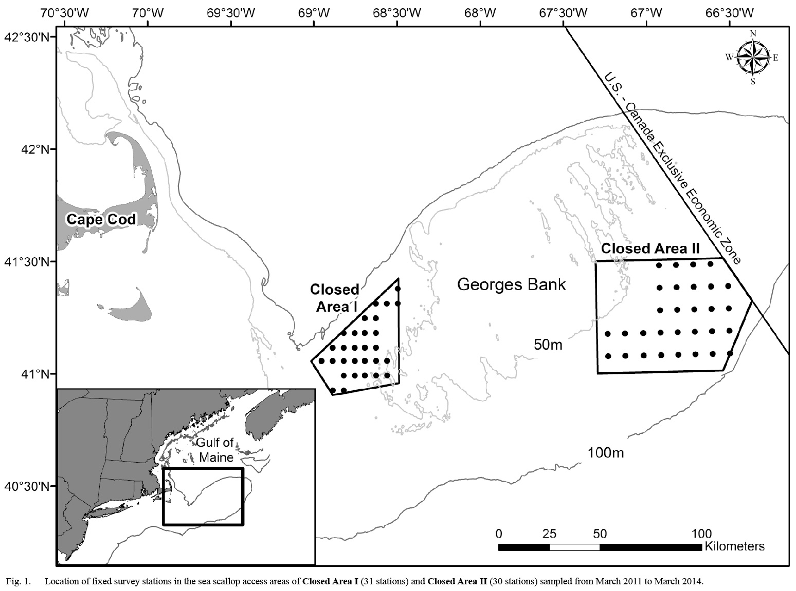
Fig. 1. |
In particular, catches of yellowtail flounder (Limanda ferruginea) have impacted the timing, location, and, ultimately, the allowable harvest of sea scallops over the past fifteen years (O’Keefe and DeCelles, 2013). The current regulatory framework mandates a strict accounting of fishery-specific bycatch. If the fleet exceeds its annual catch limit for a given species, accountability measures are implemented (e.g. in-season closures or quota reductions to account for previous overages; Magnuson-Stevens Fishery Conservation and Management Act; USDOC/NOAA/NMFS, MS 2007). Since 1999, the scallop fleet has been allocated an annual catch limit of Georges Bank yellowtail flounder. Between 1999 and 2009, in-season closures on Georges Bank have occurred several times due to yellowtail overages, resulting in economic losses to the fleet (O’Keefe and DeCelles, 2013). In addition to yellowtail flounder, bycatch of windowpane and winter flounder has also become a management concern in the scallop fishery; an accountability measure for windowpane was recently implemented in the mid-Atlantic (NEFMC, MS 2014). Although accountability measures for flatfish species other than yellowtail are not currently in place for the fishery on Georges Bank, it is plausible they may soon follow.
Given the economic consequences of scallop fishery closures due to yellowtail bycatch (O’Keefe and DeCelles, 2013), numerous efforts to mitigate the fleet’s impact on non-target species have been implemented. The fishery funds its own observer program, and has invested heavily in approaches aimed at both reactive (e.g. real-time bycatch avoidance; O’Keefe and DeCelles, 2013) and proactive strategies (e.g. gear modifications; Davis et al., MS 201) to reduce bycatch. However, the current overfished status of the Georges Bank yellowtail flounder stock (TRAC, MS 2014) and the resulting low annual allocation to the scallop fleet (which was reduced by over 40% in 2014; NEFMC, MS 2014) means that existing approaches to bycatch reduction may not be sufficient to avoid exceeding catch limits.
Documented seasonal variation in flatfish bycatch rates (Bachman, MS 2009) suggests that targeted time-area closures may be a viable option for the scallop fishery on Georges Bank. Given the relatively stationary nature of scallops (Hart and Chute, 2004) and the migratory patterns of the three flatfish species (Chang et al., 1999; Johnson et al., 1999; Pereira et al., 1999), it is plausible that periods of relative spatial segregation between target and non-target species could be identified based on spatiotemporal patterns in bycatch rates. However, the resolution of the data available is limited. Under the current management strategy, scallop access areas are only open to the fleet during certain periods of designated years, which limits the utility of fishery-dependent data for discerning seasonal trends in bycatch rates. Although the National Marine Fisheries Service-Northeast Fisheries Science Center biannual bottom trawl survey provides a continuous time series of fisheries-independent data for Georges Bank since 1963 (Despres-Patanjo et al., 1988), the survey is not conducted at the spatial resolution or temporal frequency required to assess seasonal patterns in flatfish distributions within the access areas.
To collect the fine-scale, fishery-independent information needed to better understand the spatial and temporal dynamics of flatfish bycatch in the sea scallop fishery in Closed Areas I and II on Georges Bank, a seasonal dredge survey was conducted from 2011–2014. Generalized additive mixed models (Wood, 2006, 2011), which provide a flexible framework for the investigation of spatially continuous, non-linear trends (Swartzman et al., 1992; Augustin et al., 2013), were used to identify spatiotemporal patterns in flatfish bycatch rates. The results are considered in the context of possible time-area management strategies for the Georges Bank scallop access areas.
Materials and Methods
Survey Design
Twenty-nine survey trips were conducted aboard eighteen commercial sea scallop vessels from 2011 to 2014. Survey trips were conducted monthly from March through November of 2011, and every six weeks from January 2012 to March 2014. Sampling locations in Closed Area I and Closed Area II were selected using a fixed station, systematic grid design to ensure uniform spatial coverage of each area (Fig. 1). However, some portions of each closed area could not be sampled due to bottom type (e.g. rocky substrate) or high densities of sand dollars (Echinarachnius parma. In order to evenly distribute sampling effort to areas with different spatial extents, the distance between stations in each area varied. In Closed Area I (CAI), the 31 stations were separated by 5.4 km east to west and 7.2 km north to south. The 30 stations in Closed Area II (CAII) were separated by 8.6 km east to west and 11.1 km north to south.
On each trip, the vessel was outfitted with two commercial scallop dredges: one standardized 4.6 m wide Turtle Deflector Dredge (TDD) and one 4.6 m wide New Bedford-style dredge, which was supplied by the vessel. Each dredge had 10.2 cm rings and a 25.4 cm mesh twine top, but the TDD had a modified headbale designed to exclude sea turtles (Smolowitz et al., 2012). A more detailed description of the dredges used in this fishery as well as a description of the TDD frame is provided in Smolowitz et al. (2012). Only catch data from the standardized TDD used over the entire course of the survey are presented herein. It is important to note that the large mesh used on commercial scallop dredges has a low selectivity for small flatfish (Legault et al., MS 2010). Thus, the flatfish bycatch rates observed during the course of our survey are considered to be representative only of the portion of the population available and vulnerable to capture in commercial scallop dredges.
At each station, standardized survey protocol specified that the vessel operator pass through the center of each grid cell at some point during the tow; tow direction was left to the discretion of the operator. The target tow duration was 30 minutes, with a minimum acceptable tow time of 20 minutes. Tows shorter than 20 minutes or those with gear or other operational issues were deemed invalid, and the station was resampled until an acceptable tow was completed. Target tow speed was 4.8 knots, and dredges were towed with a 3:1 wire to depth scope. Set-out and haul-back coordinates, depth, sea state, vessel speed, and weather conditions were recorded by the vessel operator. Beginning in May 2011, a temperature (Vemco Minilog) and a temperature-depth logger (Star-Oddi DST milli-TD) were attached to the dredge and programmed to acquire data every 30 seconds.
Following each tow, the catch from each dredge was sorted by species. All yellowtail, winter, and windowpane flounder were counted and measured to the nearest cm. Bycatch rates for each flatfish species in each tow were expressed in terms of catch per unit effort (CPUE) as the ratio of the number of fish caught in the TDD and the time of the tow in minutes; CPUE values for tows that varied around the target tow duration of 30 minutes were scaled accordingly.
Seasonal trends in flatfish catches
Generalized additive mixed models (GAMMs; Wood, 2006, 2011) were used to investigate seasonal changes in the spatial distribution of flatfish catches. There were a large number of tows with zero flatfish catch in both areas (Table 1). Therefore, a Tweedie error distribution (which can accommodate continuous data with many zeros; Tweedie, 1984; Dunn and Smyth, 2005) and a log link function were assumed (Candy 2004; Shono 2008). The Tweedie distribution belongs to the family of exponential dispersion models, which generalize the exponential families used in generalized linear and additive modeling frameworks (Jørgensen 1992). The variance of a Tweedie-distributed random variable, Y, is given by Var(Y) =φ [E(Y)]p, where φ is a dispersion parameter and p is the Tweedie index parameter, which is a constant. When p is equal to 0, 1, or 2, the Tweedie is equivalent to the normal, Poisson, or gamma distribution, respectively. For values of p between 1 and 2, the model is a compound Poisson-gamma distribution. When p is closer to 1, the Tweedie distribution most closely resembles the Poisson and allows for a point mass at 0; as the value of p increases, the Tweedie more closely approximates the gamma (Candy 2004).
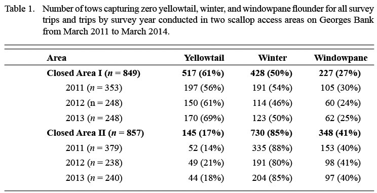
Table 1 |
Because we were most interested in describing the spatial distribution of catches over the course of the year, we chose to model catch rates as a function of geographic location and month rather than environmental conditions. Additionally, depth and bottom temperature (the two available environmental variables we expected to correlate most highly with catch rates; Swartzman et al., 1992; Hyun et al., 2014) were not collected over the entire course of the survey and were highly correlated with longitude and month, respectively. Preliminary analyses also indicated that the results of models based on those covariates did not adequately describe the distribution of residuals; they are therefore not presented further here. For model fitting, tow location was estimated as the midpoint of the great circle distance between the start and end points of each tow using the “geosphere” package (Hijmans et al., 2012) in R (R Core Team, 2015). Midpoint coordinates were projected into the universal transverse Mercator coordinate system (UTM zone 19) using the R package “rgdal” (Bivand et al., 2013). Although we used standardized sampling protocols on each survey, different vessels were employed over the course of the study. Therefore, vessel was incorporated as a random effect to account for variability due to differences in vessel handling, engine power, or other technical characteristics of the vessels employed, as well as other inter-vessel differences not accounted for by the covariates of interest (Candy 2004; Augustin et al., 2013).
The response, the CPUE of each flatfish species for tow j from vessel i (yij) was modelled as:
,
where β0 is an intercept term; f1 is a smooth function of the covariates associated with vessel i and tow j; northing and easting are projected tow coordinates; β1 is a coefficient specifying the effect of survey year (note the distinction from calendar year); vi represents the random effect of vessel; and εij is an independently and identically distributed (i.i.d.) error term. It was assumed that vi~Normal(0,σi2) and i.i.d. The incorporation of vessel as a random effect term allows for marginal, “population-level” (i.e. vessel-averaged) predictions via integration of vi out of the conditional CPUE predictions (Candy 2004; Augustin et al., 2013).
 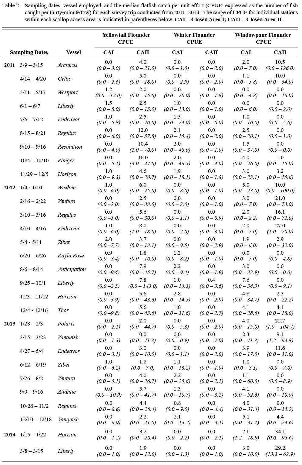
Table 2 |
Shifts in the spatial distribution of the catch by month are represented by f1, which is a tensor product interaction of a two-dimensional isotropic smooth for location and a one-dimensional smooth for month. The tensor product construction of this interaction term allows for CPUE to be modeled as a smooth function of location and month while being invariant to their relative scaling (Wood, 2006). Thin plate regression splines (Wood, 2006) were used to represent CPUE as a function of geographic coordinates (northing and easting). A cyclic cubic regression spline was used to represent trends in CPUE by month to avoid discontinuities between December and January (Zuur et al., 2009). Catches of winter flounder in CAII were too low (Table 2, Fig. 2; observed CPUE < 4.4 fish per tow in all cases; 3rd quantile = 0.0 fish per tow) and diffuse to se nsibly model in the framework used, as confirmed by residual diagnostics. Therefore, only the results for winter flounder catches in CAI are presented.
Given that stations in CAI and CAII were separated by approximately 100 km, two unique models were constructed for CAI and CAII to avoid smoothing over areas that were not sampled. Simpler models nested within the above equation (e.g. models without month, models with the interaction term between geographic location and month replaced by additive effects; see Tables 3–5 for the full list of models fitted) were also considered. For each species, the Tweedie index parameter (p) was set to the value that maximized the penalized log-likelihood for all model variants (Tables 3–5). All models were fitted via maximum likelihood estimation using the R package “mgcv” (Wood, 2006, 2011).
 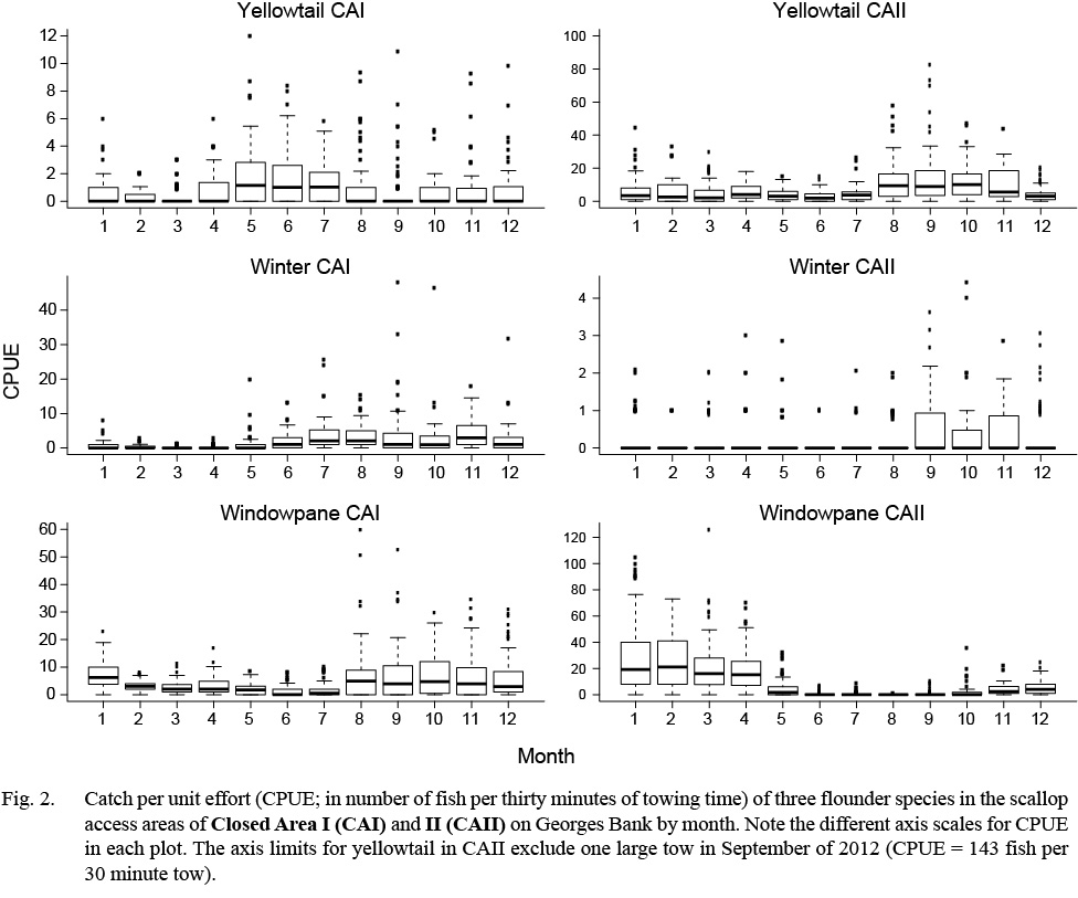
Fig. 2. |
Model selection and spatial prediction
Model fit was evaluated based on the Akaike Information Criterion (AIC; Akaike, 1973). Interaction and individual terms were retained in the model if their inclusion resulted in lower AIC values and explained a higher proportion of the deviance. The AIC difference (Δi) of each model was calculated based on the lowest observed AIC value (AICmin) as Δi = AICi - AICmin. Models with Δi < 2 were considered indistinguishable in terms of fit (Burnham and Anderson, 2002). Residual plots were examined to assess model fit.
 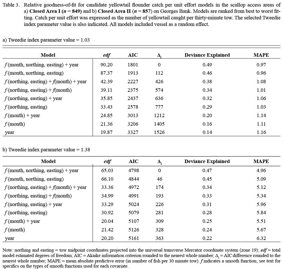
Table 3 |
While location and time were included explicitly in the full models, there was still the possibility of unexplained residual correlation. Therefore, model fit was also assessed based on the mean absolute prediction error (MAPE) to corroborate the likelihood-based AIC approach (Augustin et al., 2013). Because the CPUE of each species varied widely over the course of the year, we chose to use the MAPE rather than the root mean square predictive error, which is more sensitive to large values (Willmott and Matsuura, 2005). Observed data were split into ten test sets based on randomly sampling fixed station locations. For each test set, models were fitted to the remaining data. Values predicted for the omitted set were then compared to observed values to estimate predictive error. The MAPE for each set was calculated as:
 . .
 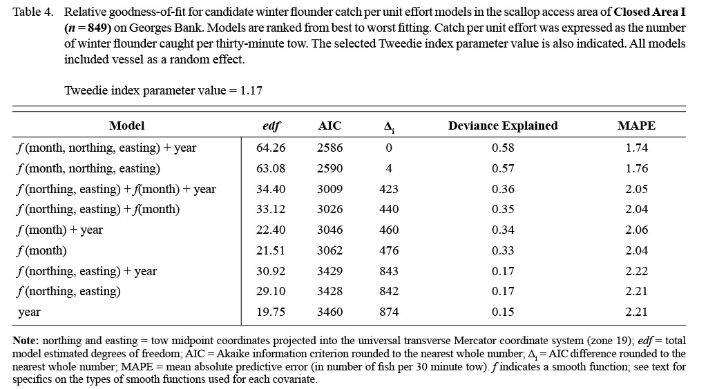
Table 4 |
The ten resulting MAPE values were then averaged to generate an overall MAPE for each model.
The spatially explicit models used herein produce a smooth surface from which the expected flatfish CPUE can be estimated at any location within the study area. For models that included year as a fixed effect, the reference level was set to the last survey year (2013) for prediction. In instances when the best fitting models included geographic coordinates, prediction areas were roughly bounded based on the distribution of tow midpoints to avoid extrapolation into unsampled areas (Augustin et al., 1998). The expected flatfish CPUE was predicted over a high resolution grid (10 000 cells in each closed area). As our aim was to identify bycatch hotspots rather than to predict the number of flatfish that would be caught in a given tow, we decided to plot our estimates at this scale to ease interpretation. However, it is important to note that such fine-scale estimates would be prone to bias if used as the basis for field predictions of actual catches.
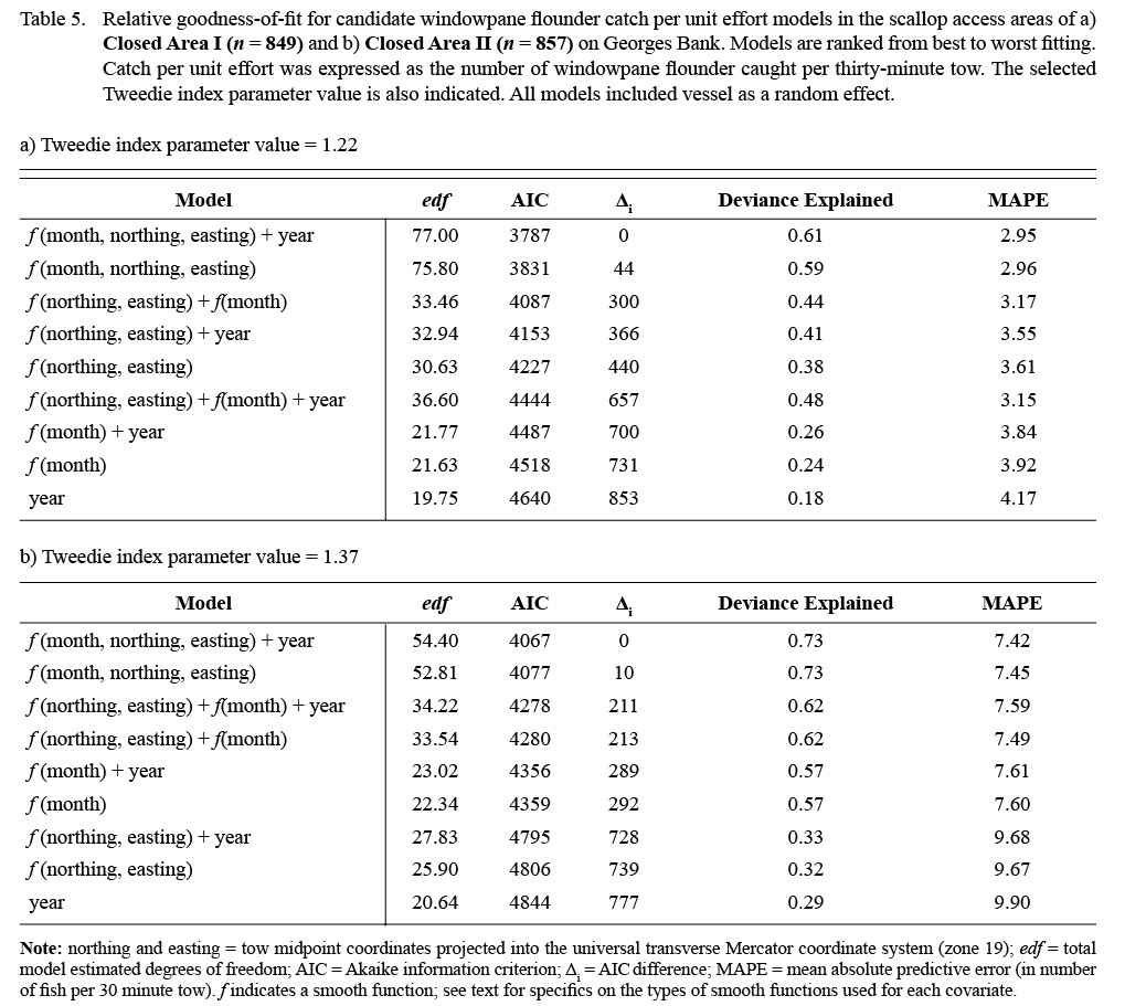
Table 5 |
Results
A total of 1 706 valid tows were completed from March 2011 to March 2014 (Table 2). Over the 29 survey trips, a total of 6 852 yellowtail flounder, 1 754 winter flounder, and 12 202 windowpane flounder were collected in the TDD. Catches of all three flounder species varied substantially between areas and seasons (Table 2; Fig. 2). Yellowtail and windowpane flounder catches were generally higher in CAII, with the greatest number of yellowtail caught in the fall and windowpane in the winter and spring (Fig. 2). Winter flounder catches were generally low throughout the year in both areas, but were highest in CAI in the summer and fall (Fig. 2). Yellowtail CPUE ranged from 0.0 to 12.0 in CAI and 0.0 to 143.0 in CAII. The CPUE of winter flounder and windowpane ranged from 0.0 to 48.0 and from 0.0 to 60.0 in CAI, respectively. In CAII, CPUE of winter flounder ranged from 0.0 to 4.4 and windowpane from 0.0 to 126.0.
Seasonal trends in flatfish catches
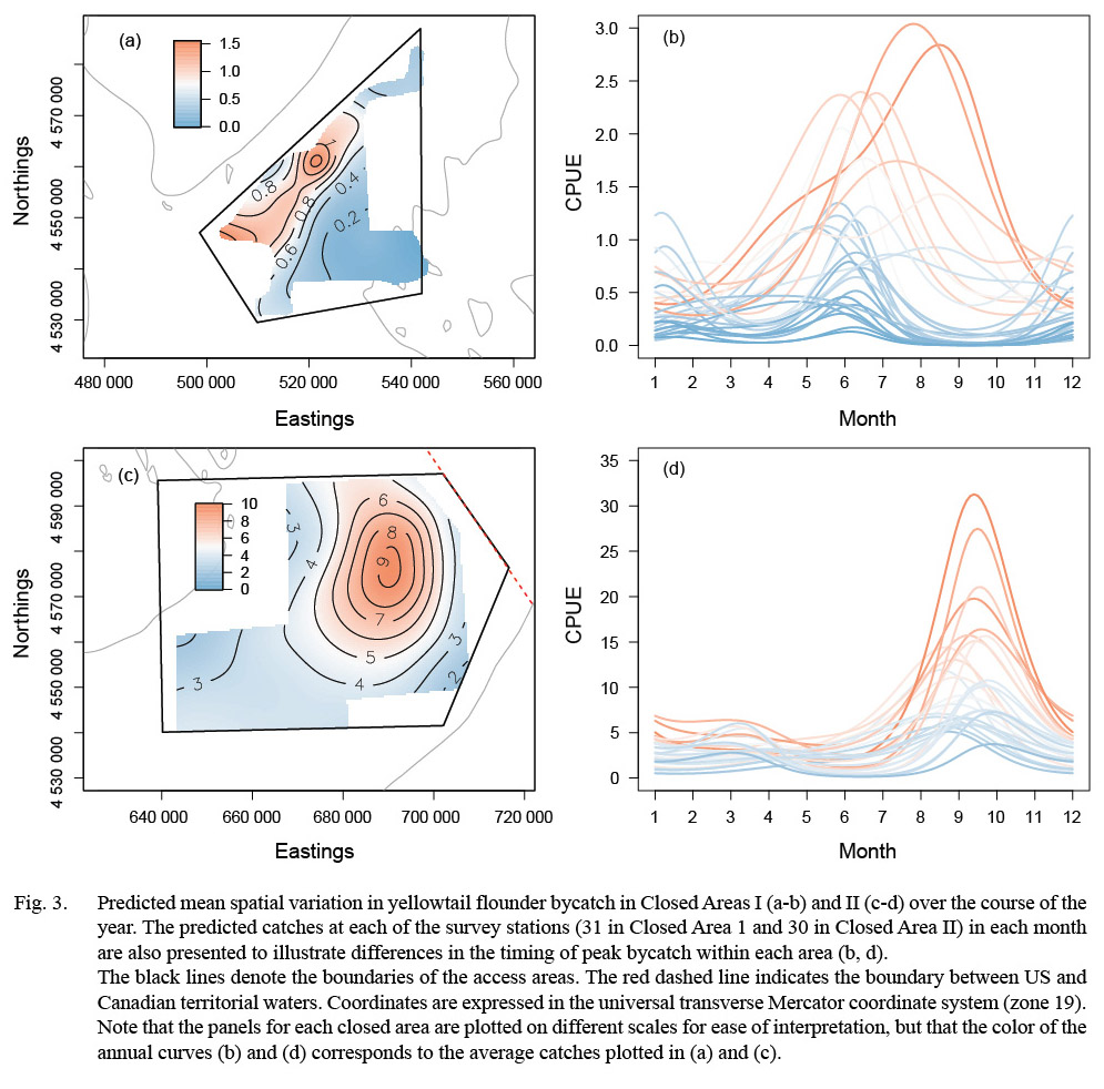
Fig. 3. |
The results of the GAMM analyses provided insight into the spatial distribution underlying the monthly trends in flatfish catches for each area. Variation in the CPUE of all three species was best described by models including the month-location smoother, indicating difference in the spatial distribution of flatfish catches by month (Tables 3–5). In all cases, the best fitting models also included survey year as a factor, suggesting differences in the magnitude of catches between years; however, differences in fit between the models including both survey year and the month-location smoother and those only including the month-location smoother were generally minimal (Tables 3–5). Model comparisons based on MAPE estimates supported the model selected based on AIC ranking in all cases (Tables 3–5). In general, the selected models explained a large proportion of the observed variance (deviance explained 0.47 to 0.73 for all cases; Tables 3–5), and residual plots indicated that the assumptions and the selected values of the Tweedie index parameter were appropriate.
For yellowtail, model results for both closed areas suggested changes in the distribution and magnitude of bycatch by month (Fig. 3). In CAI, predicted CPUE was generally low in all months (mean CPUE < 2.0 fish per 30 minute tow for all locations) but was highest along the northwestern boundary from the spring into the fall (Fig. 3a-b). Catches in CAII exhibited greater variation over the year (Fig. 3c-d). The predicted CPUE was relatively low over large portions of CAII, with localized areas of higher catch (CPUE > 15.0) in the eastern portion of CAII during the fall (Fig. 3c-d). Predicted catches in both areas were lower in survey year 2013 than in the previous years (Table 6).
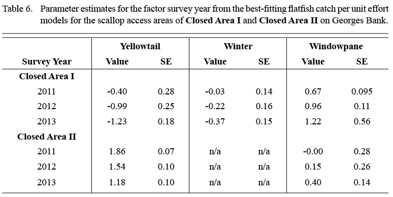
Table 6 |
Model results also suggested seasonal changes in the distribution of winter flounder in CAI. Winter flounder were largely absent in predicted catches from February to April (Fig. 4). Predicted catches were highest along the northwestern and southern portions of the area from July to November (CPUE > 5.0; Fig. 4). The best fitting model suggested that predicted catches in CAI were lower in 2013 than in survey years 2011 and 2012 (Table 6).
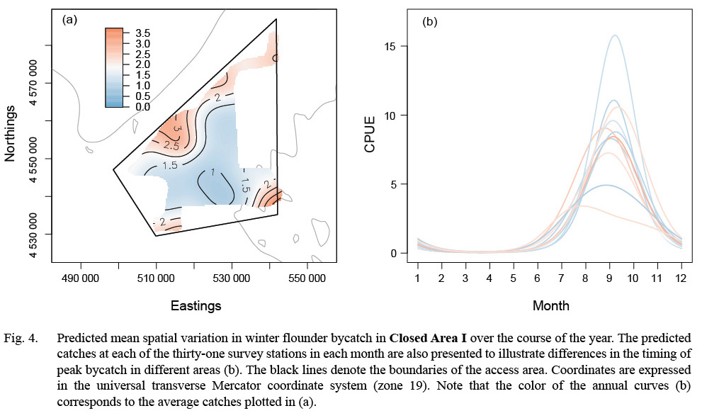
Fig. 4. |
Monthly variation in the predicted bycatch of windowpane flounder was greater than for the other two species (Fig. 5). The predicted range of windowpane catches was greater in CAII (CPUE: 0.0–69.9) than CAI (CPUE: 0.0–30.2) but was more episodic in CAII. In CAI, the highest predicted catches occurred in the southeastern portion of the area in the fall (September to December; Fig. 5a-b). The highest predicted catches in CAII occurred from January to April, and were relatively high over almost the entire area surveyed (Fig. 5c-d). From May to August, windowpane bycatch in CAII appeared to be minimal (Fig. 5c-d). Predicted catches in both areas were higher in survey year 2013 than in the previous two survey years (Table 6).
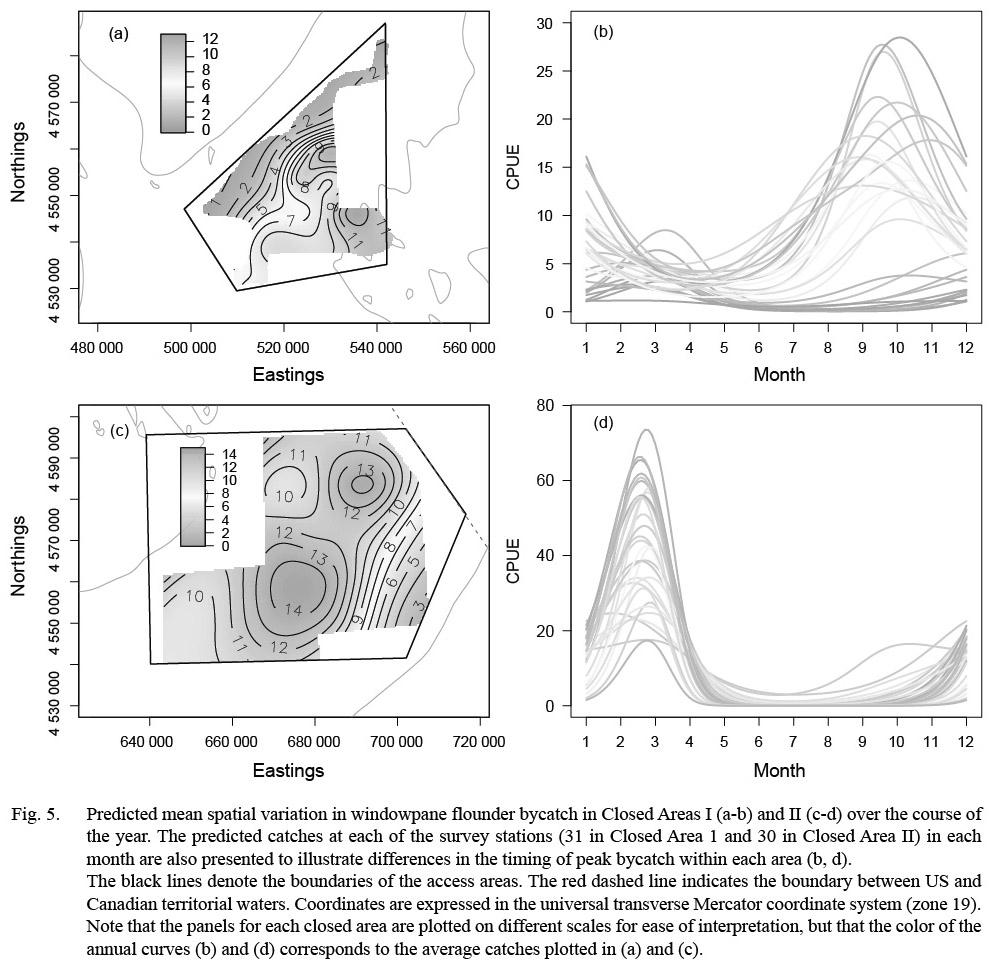
Fig. 5. |
Discussion
The results of our three-year dredge survey revealed considerable spatiotemporal variation in flatfish bycatch both within and between two scallop access areas on Georges Bank. By frequently sampling Closed Areas I and II over an extended period of time, we were able to document localized, seasonal shifts in the bycatch rates of three flatfish species. Our results suggest consistent seasonal patterns in flatfish bycatch that may help managers identify the optimal times to open the access areas to the scallop fleet in order to reduce bycatch of yellowtail, winter, and windowpane flounder.
The selected models for flatfish bycatch explained a high degree of the variability observed over the three years of the survey. This was not surprising given our use of GAMMs, which allow for flexible, non-linear fits to explanatory variables (Wood, 2006). Additionally, by modeling bycatch rates as a function of location, which is inherently correlated with other factors (e.g. depth, bottom temperature, prey availability, substrate type), we were able to encompass a myriad of potential mechanistic drivers without explicitly including them in the model structure. While this certainly compromises a more holistic understanding of the observed trends, as well as the long-term predictive power of the models applied herein, we were most interested in identifying seasonal changes to inform management.
Though we did not directly investigate the effect of environmental factors on bycatch, similar studies conducted in other regions may provide insight into the seasonal trends we characterized. Swartzman et al. (1992) used spatially-explicit GAMs to investigate inter-annual trends and environmental effects on flatfish catches from trawl survey data in the Bering Sea. They found that models based only on temperature and depth explained nearly as much of the observed variation in the spatial distribution of most species as did the models incorporating geographic coordinates. Limited information is available regarding environmental correlates to flatfish catch rates in CAI and CAII, but temperature and depth likely influence the spatial distribution of yellowtail, winter, and windowpane flounder in a similar fashion (Hyun et al., 2014). Habitat type may also be an important factor. Yellowtail and windowpane flounder typically occur on sand or sand-mud substrates (Chang et al., 1999; Johnson et al., 1999), such as those found along the southeastern edge of the access area in CAII (Murawski et al., 2000). Winter flounder occupy sandy substrates as well, but are more often associated with the mixed sand-gravel sediments typical of CAI (Pereira et al., 1999; Murawski et al., 2000).
Alternatively, environmental covariates may operate via indirect effects by modifying the distribution and behavior of prey species, or by influencing the timing of flatfish migration to feeding or spawning grounds (Kotwicki et al., 2005). All three flatfish species are known to make seasonal migrations in response to both abiotic and biotic factors over some portion of their range (Chang et al., 1999; Johnson et al., 1999; Pereira et al., 1999). The survey CPUEs of all three species were relatively low during periods of peak spawning on Georges Bank (yellowtail flounder spawn from May to August, winter flounder from March to May, and windowpane from June to October; O’Brien et al., MS 1993), suggesting that neither area serves as a primary spawning ground for the species. Maturity data collected during the course of the survey corroborate this, as few flounder were observed to be in spawning condition (C. Huntsberger, unpublished data).
Whatever the driving mechanisms may be, the spatio-temporal patterns of flatfish bycatch documented herein may be useful in terms of optimizing the harvest of sea scallops while avoiding bycatch, and hence accountability measures, in the Atlantic sea scallop fishery on Georges Bank. It is important to note that our results are only suggestive of relative trends in the availability of flatfish species to the scallop fishery, and are not necessarily related to actual trends in abundance in the two areas surveyed, particularly given the potential impact of large tows on estimated trends (Maunder et al., 2006). However, our results do suggest that predictable seasonal patterns in flatfish bycatch may provide a practical foundation for the formulation of effective time-area management strategies. Based in part on the survey results reported herein, CAII is now closed to the scallop fleet from August through November (NEFMC, MS 2013) in an effort to reduce high rates of yellowtail bycatch.
Acknowledgements
The authors thank the vessel owners, operators, and crew members of the F/Vs Anticipation, Arcturus, Atlantic, Celtic, Endeavor, Horizon, Kayla Rose, Liberty, Polaris, Ranger, Regulus, Resolution, Thor, Vanquish, Venture, Westport, Wisdom, and Zibet, who made this project possible. They are also grateful to survey staff from Coonamessett Farm Foundation (in particular F. Davis, B. Valenti, M. Weeks), the University of Massachusetts Dartmouth (E. Adams, C. Bank, A.Barkley, J. Garrity, S. Inglis, M. Levesque, R. Malloy, D. Zemeckis), the Virginia Institute of Marine Science (W. DuPaul), and Northeastern University (S. Heck). D. Kulka, D. Keith, and one anonymous reviewer provided helpful comments on an earlier draft of this manuscript. This study was funded by NOAA Sea Scallop Research Set-Aside grants NA11NMF4540021, NA12NMF4540034, and NA13NMF4540011.
References
AKAIKE, H. 1973. Information theory as an extension of the maximum likelihood principle. In: Second international symposium on information theory. B.N. Petrov and F. Csaki (eds.). Akademiai Kiado, Budapest, Hungary, p. 267–281.
AUGUSTIN, N. H., D. L. BORCHERS, E. D. CLARKE, S. T. BUCKLAND, and M. WALSH. 1998. Spatiotemporal modelling for the annual egg production method of stock assessment using generalized additive models. Can. J. Fish. Aquat. Sci. 55(12): 2608–2621. doi.org/10.1139/f98-143
AUGUSTIN N. H., V. M. TRENKEL, S. N. WOOD, and P. LORANCE. 2013. Space-time modelling of blue ling for fisheries stock management. Environmetrics 24(2): 109–119. doi.org/10.1002/env.2196
BACHMAN, M. S. MS 2009. Determinants of yellowtail flounder bycatch in the Closed Area II scallop access fisheries on Georges Bank. MS Thesis. University of Massachusetts Dartmouth.
BIVAND, R., T. KEITT, and B. ROWLINGSON. 2013. rgdal: Bindings for the geospatial data abstraction library. R package version 0.8–14. http://CRAN.R-project.org/ package=rgdal
BURNHAM, K. P., and D. R. ANDERSON. 2002. Model selection and multimodel inference: a practical information-theoretic approach. Springer, New York.
CANDY, S. G. 2004. Modelling catch and effort data using generalised linear models, the Tweedie distribution, random vessel effects and random stratum-by-year effects. CCAMLR Science, 11: 59–80.
CHANG, S., P. L. BERRIEN, D. L. JOHNSON, and W. W. MORSE. 1999. Essential fish habitat source document: windowpane, Scophthalmus aquosus, life history and habitat characteristics. NOAA Tech. Mem., NMFS-NE-137.
DAVIS, F., M. WINTON, C. PARKINS, and D. RUDDERS. MS 2014. Testing of scallop dredge bag design changes for flatfish bycatch reduction. Coonamessett Farm Foundation Final Report, Scallop Research Set-Aside, 48 p.
DESPRES-PATANJO, L. I., T. R. AZAROVITZ, and C. J. BYRNE. 1988. Twenty-five years of fish surveys in the northwest Atlantic: the NMFS Northeast Fisheries Center’s bottom trawl survey program. Mar. Fish. Rev., 50(4): 69–71.
DUNN, P. K., and G. K. SMYTH. 2005. Series evaluation of Tweedie exponential dispersion model densities. Stat. Comput. 15: 267–280. doi.org/10.1007/s11222-005-4070-y
HART, D. R., and A. S. CHUTE. 2004. Essential fish habitat source document: sea scallop, Placopecten magellanicus, life history and habitat characteristics, second edition. NOAA Tech. Mem., NMFS-NE-189.
HIJMANS, R. J., E. WILLIAMS, and C. VENNES. 2012. geosphere: Spherical Trigonometry. R package version 1.2-28. URL http://CRAN.R-project.org/package=geosphere
HYUN, S., S. X. CADRIN, and S. ROMAN. 2014. Fixed and mixed effects models for fishery data on depth distribution of Georges Bank yellowtail flounder. Fish. Res. 157: 180–186. doi.org/10.1016/j.fishres.2014.04.010
JOHNSON, D. L., W. W. MORSE, P. L. BERRIEN, and J. J. VITALIANO. 1999. Essential fish habitat source document: yellowtail flounder, Limanda ferruginea, life history and habitat characteristics. NOAA Tech. Mem., NMFS-NE-140.
JØRGENSEN, B. 1992. Exponential dispersion models and extensions: a review. Int. Stat. Rev. 60(1): 5–20. doi.org/10.2307/1403498
KOTWICKI, S., T. W. BUCKLEY, T. HONKALEHTO, and G. WALTERS. 2005. Variation in the distribution of walleye Pollock (Theragra chalcogramma) with temperature and implications for seasonal migration. Fish. Bull. 103: 574–587.
LEGAULT, C. M., D. B. RUDDERS, and W. D. DUPAUL. MS 2010. Yellowtail flounder catch at length by scallop dredges: A comparison between survey and commercial gear. Transboundary Resource Assessment Committee, Reference Document 2010, 9 p.
MAUNDER, M. N., J. R. SIBERT, A. FONTENEAU, J. HAMPTON, P. KLEIBER, and S. J. HARLEY. 2006. Interpreting catch per unit effort data to assess the status of individual stocks and communities. ICES J. Mar. Sci. 63: 1373–1385. doi.org/10.1016/j.icesjms.2006.05.008
MURAWSKI, S. A., R. BROWN, H. L. LAI, P. J. RAGO, and L. HENDRICKSON. 2000. Large-scale closed areas as a fishery-management tool in temperate marine systems: the Georges Bank experience. B. Mar. Sci. 66(3): 775–798.
NEW ENGLAND FISHERY MANAGEMENT COUNCIL (NEFMC). MS 2003. Final Amendment 10 to the Atlantic Sea Scallop Fishery Management Plan with a supplemental environmental impact statement, regulatory impact review, and regulatory flexibility analysis. Newburyport, MA, 1113 p. Available at www.nefmc.org/scallops/index.html
MS 2013. Final Framework 24 to the Atlantic sea scallop fishery management plan and Framework 49 to the multispecies fishery management plan including a draft environmental assessment, an initial regulatory flexibility analysis, and stock assessment and fishery evaluation (SAFE report). Newburyport, MA, 354 p. Available at www.nefmc.org/scallops/index.html
MS 2014. Final Framework 25 to the Atlantic sea scallop fishery management plan including a final environmental assessment, an initial regulatory flexibility analysis, and stock assessment and fishery evaluation (SAFE report). Newburyport, MA, 319 p. Available at www.nefmc.org/scallops/index.html
NORTHEAST FISHERIES SCIENCE CENTER (NEFSC). MS 2010. 50th Northeast Regional Stock Assessment Workshop (50th SAW) Assessment Report. U.S. Dept. Commer., Northeast Fish. Sci. Cent. Ref. Doc. 10–17, 844 p.
O’BRIEN, L., J. BURNETT, and R. K. MAYO. MS 1993. Maturation of nineteen species of finfish off the northeast coast of the United States, 1985–1990. NOAA Technical Report NMFS 113, 66 p.
O’KEEFE, C. E., and G. R. DECELLES. 2013. Forming a partnership to avoid bycatch. Fisheries 38: 434–444. doi.org/10.1080/03632415.2013.838122
PEREIRA, J. J., R. GOLDBER, J. J ZISKOWSKI, P. L. BERRIEN, W. W. MORSE, and D. L. JOHNSON. 1999. Essential fish habitat source document: winter flounder, Pseudopleuronectes americanus, life history and habitat characteristics. NOAA Tech. Mem., NMFS-NE-138.
R CORE TEAM. 2015. R: A language and environment for statistical computing. R Foundation for Statistical Computing, Vienna, Austria. URL www.R-project.org/
SHONO, H. 2008. Application of the Tweedie distribution to zero-catch data in CPUE analysis. Fish. Res. 93: 154–162. doi.org/10.1016/j.fishres.2008.03.006
SMOLOWITZ, R., H. O. MILLIKEN, and M. WEEKS. 2012. Design, evolution, and assessment of a sea turtle deflector dredge for the U.S. Northwest Atlantic sea scallop fishery: impacts on fish bycatch. N. Am. J. Fish. Manage. 32(1): 65–76. doi.org/10.1080/02755947.2012.661386
SWARTZMAN, G., C. HUANG, and S. KALUZNY. 1992. Spatial analysis of Bering Sea groundfish survey data using generalized additive models. Can. J. Fish. Aquat. Sci. 49: 1366–1378. doi.org/10.1139/f92-152
TRAC. MS 2014. Georges Bank Yellowtail Flounder. TRAC Status Report 2014/03.
TWEEDIE, M. C. K. 1984. An index which distinguishes between some important exponential families. In: Statistics: applications and new directions. Proceedings of the Indian Statistical Institute Golden Jubilee International Conference. J.K. Ghosh and J. Roy (eds.) Indian Statistical Institute, Calcutta, p. 579–604.
U.S. DEPARTMENT OF COMMERCE, NATIONAL OCEANIC AND ATMOSPHERIC ADMINISTRATION, and NATIONAL MARINE FISHERIES SERVICE (USDOC/NOAA/NMFS). MS 2007. Magnuson-Stevens Fishery Conservation and Management Act, as amended through January 12, 2007. Public Law 94–265, 170 p.
VAN VOORHEES, D. (ed.). 2014. Fisheries of the United States, 2013. NMFS Office of Science and Technology, Fisheries Statistics Division, Silver Spring, Maryland, August 2014, 129 p.
WILLMOTT, C. J., and K. MATSUURA. 2005. Advantages of the mean absolute error (MAE) over the root mean square error (RMSE) in assessing average model performance. Climate Res. 30: 79–82. doi.org/10.3354/cr030079
WOOD, S. N. 2006. Generalized additive models: an introduction with R. Chapman and Hall/CRC, Boca Raton, FL.
2011. Fast stable restricted maximum likelihood and marginal likelihood estimation of semiparametric generalized linear models. J. Roy. Stat. Soc B 73(1): 3–36. doi.org/10.1111/j.1467-9868.2010.00749.x
ZUUR, A. F., E. N. IENO, N. J. WALKER, A. A. SAVELIEV, and G. M. SMITH. 2009. Mixed effects models and extensions in ecology with R. Springer, New York, NY. doi.org/10.1007/978-0-387-87458-6
|