J. Northw. Atl. Fish. Sci., Vol. 51: 15–31
Cameron T. Hodgdon1,3, Michael Torre1,2, and Yong Chen1
1University of Maine, School of Marine Sciences, Orono, ME 04469, USA
2University of Washington, School of Aquatic and Fishery Sciences, Seattle, WA 98195, USA
3Corresponding Author’s Present Institution and Address: University of Maine, School of Marine Sciences, 5741 Libby Hall Room 221, Orono, ME 04469, USA
Cameron T. Hodgdon’s Email (Corresponding Author): cameron.hodgdon@maine.edu
Michael Torre’s Email: michael.torre@maine.edu
Yong Chen’s Email: ychen@maine.edu
Hodgdon, C.T., Torre, M., and Chen, Y. 2020. Spatiotemporal variability in Atlantic sea scallop (Placopecten magellanicus) growth in the Northern Gulf of Maine. J. Northw. Atl. Fish. Sci., 51: 15–31. https://doi.org/10.2960/J.v51.m729
Abstract
Simulation-based assessment tools coupled with large-scale and consistent monitoring efforts contribute to the overall success of the Atlantic sea scallop (Placopecten magellanicus; ASC) fishery on the North American east coast. However, data from the Northern Gulf of Maine (NGOM) are usually excluded from the assessment because limited monitoring effort and an overall lack of information regarding the growth of ASCs in this region have led to large uncertainty of fine-scale dynamics. The objectives of this study are to determine if ASC growth varies spatially and/or temporally across the NGOM and if the variation in growth can be explained in part by variability in bottom temperature and bottom salinity. To achieve these objectives, ASC shells have been continually collected through a partnership between the University of Maine and Maine Department of Marine Resources since 2006. Individualistic ASC length-at-age curves are developed to evaluate small and large scale spatio-temporal variabilities. In comparison to ASC growth on Georges Bank and in Southern New England, it appears that ASCs in the NGOM are growing at a similar rate yet have the potential to grow to a larger size. No clear spatio-temporal trends in ASC growth are identified in the NGOM. However, our analysis reveals that bottom temperature and bottom salinity may be influencing inter-annual variabilities and contribute to growth rate differences seen between locations and years. This may imply changes in ASC growth in the future with increasing warming in the Gulf of Maine.
Keywords: Atlantic sea scallop, Environmental drivers, Gulf of Maine, Von Bertalanffy growth parameters
Download Citation Data

Citation to clipboard
 Reference management software (Endnote, Mendeley, RefWords, Zotero & most other reference management software)
LaTex, BibDesk & other specific software
Introduction
The Atlantic sea scallop (Placopecten magellanicus; ASC) is a historically important commercial bivalve on the North American east coast. In the United States, ASCs are harvested from Cape Hatteras, North Carolina to Cobscook Bay, Maine (Hart and Chute, 2004). ASC biomass (in metric tons of meat) has more than doubled in the last decade over their range (NEFSC 2018) and ASCs are not overfished and overfishing is not occurring (NEFSC, 2018). This is due largely to extant and detailed approaches used to manage this fishery on a large-scale level. Techniques have been developed that allow for population-wide simulations under different fishing scenarios to determine catch limits per area for consecutive years (Rheuban et al., 2018; NEFSC, 2018). However, areas like the Northern Gulf of Maine (NGOM) are usually excluded from these predictive models because of lack of information regarding the growth of ASCs in these regions. More southern areas such as Georges Bank (GBK) and the Mid-Atlantic Bight (MAB) are high-production fishing grounds for this species and so the bulk of knowledge concerning ASC growth rates has been from samples collected from these areas (Hart and Chute, 2009a; Hart and Chute, 2009b; Mann and Rudders, 2019).
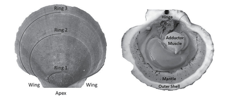
Fig. 1
A scallop is a bivalve mollusk, having two hardened calcium carbonate structures connected by a hinge and a large adductor muscle (Fig. 1). Unlike exoskeletal animals that shed their outer layers during a molt, scallops must expand their shell as they grow (Marin and Luquet, 2004). Because of this, they must constantly be laying down new material. This new material (in the form of the aforementioned calcium carbonate) is set in place on the outer edges of shells, resulting in ring formation much like trees (Hart and Chute, 2009a; Hart and Chute, 2009b). This growth allows for simple calculation of length-at-age curves (a.k.a. growth curves). The rings are formed due to seasonal changes in growth rates; with shell formation being faster in the warmer months and slower in the colder months (Côté et al., 1993; Harris and Stokesbury, 2006; Hart and Chute, 2009a; Hart and Chute, 2009b), forming a single ring per year of growth. This is due to the direct effect that environmental variables (such as temperature and salinity) have on the metabolism of the animals (Côté et al., 1993). Many studies have demonstrated linkages between the rate of ASC growth and environmental conditions such as temperature, salinity, and depth (MacDonald and Thompson, 1985a; MacDonald and Thompson, 1985b; Thouzeau et al., 1991; Harris and Stokesbury, 2006; Hart and Chute, 2009a; Chute et al., 2012), yet few studies have looked at the spatiotemporal variation of these effects at finer spatial scales than large marine ecosystems (LMEs) such as GBK and the MAB.
Climate change is causing the NGOM ecosystem to warm at an accelerated rate compared with a majority of the world’s oceans; with an average-per-year increasing temperature of 0.026˚C (Pershing et al., 2015). Bottom temperature and bottom salinity fluctuate around yearly means as seasons change, but these yearly means for both variables are rising in the face of climate change (Pershing et al., 2015; Saba et al., 2016). This means that ASC growth has the potential to change as well. If it can be understood how these environmental variables affect ASC growth in the NGOM, it can be inferred if and how their growth will change into the future.
Understanding spatiotemporal variation in growth is important for the management of any marine resource, especially those in an environment experiencing rapid environmental changes (Maunder and Piner, 2015). Mann and Rudders (2019) stated the importance of understanding age/length structures to inform the current assessment model for ASCs in GBK and the MAB, referring to using this information to enhance the current understanding of ASC recruitment and mortality. Assuming incorrect growth structures can lead to large effects on stock assessment outcomes and incorrect management advice (Maunder and Piner, 2015). Little is known about the NGOM LME as it pertains to ASC growth, accentuating the increased likelihood of wrongly assumed growth parameters. Most information about NGOM ASC growth comes from a singular study by Truesdell (2014), wherein growth is analyzed across different spatial zones in the NGOM. In short, Truesdell (2014) concluded that NGOM scallops grow to larger sizes, yet grow slower than scallops in GBK and the MAB. This study, however, only addresses spatial differences in growth and spatial effects of environmental variables.
The objectives of this study were to 1) Determine if ASC growth varies spatially and/or temporally across the four management zones in the NGOM (Fig. 2) and 2) Determine if variation in ASC growth in these areas and across years can be explained in part by bottom temperature and bottom salinity. To achieve these objectives, von Bertallanfy growth parameters for multiple locations and age classes are determined using methods from Hart and Chute (2009a) and growth increment data is used in multiple regression analyses to determine relative influence of environmental factors bottom temperature and bottom salinity as well as spatial (latitude and longitude) and time-varying (year of growth) factors. This same process to determine spatiotemporal variation and influence of environmental factors can be applied to many bivalve species whose historical size-at-age is determinable from their shells or for fish species who have reliable otolith size to fish length relationships.
Methods
Study Area
The NGOM management area (Fig. 2) is the most northern extent of the United States’ ASC stock. This area is managed on smaller scales: namely inshore (<3 nautical miles (nm) from shore) and offshore (>3nm from shore). The inshore NGOM is split into three distinct management sections: Zone 1 (commonly referred to as the Western Gulf of Maine), Zone 2 (commonly referred to as the Eastern Gulf of Maine), and Zone 3 (Cobscook Bay; Fig. 2), with each zone having slightly different management techniques, but the same management entity: the Maine Department of Marine Resources (MDMR). The offshore NGOM (referred to here as management zone 4) is treated as a single large unit and is managed jointly at both state and federal levels (by MDMR and the New England Fishery Management Council).
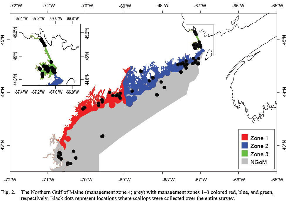
Fig. 2
The NGOM is characterized as having fluctuating yearly temperatures and salinities, influenced by a combination of the warm and salty North-bound Gulf Stream and the colder, less salty South-bound Labrador Current (Durbin et al., 2003; Wanamaker et al., 2008). Additionally, year to year variations are also present in these variables due to changing ratios of incoming water masses due to climate change (Mills et al., 2013; Pershing et al., 2015), resulting in higher observed temperatures and salinities.
Ageing and Growth Modelling
A partnership between the University of Maine and the MDMR has been responsible for collecting ASC shells from the study area since 2006 which are subsequently stored at the University of Maine until they are aged. Part of these shells were utilized for Truesdell’s (2014) analyses, but the sample size has been greatly improved in recent years with additional samples being collected from broader areas in the NGOM.
Aging of shells followed methods from Hart and Chute (2009a). Each shell is measured from the apex (center of the hinge; Fig. 1) to each consecutive ring, producing a number of data points for each scallop as there are visible rings. The number of rings, though, is not always indicative of absolute age, however. The first two years of growth of an ASC are not as predictable or uniform as from two years onward. Because of this, the one-year growth ring or the two-year growth ring may be the first visible ring. Agers are taught how to infer which year the first visible ring corresponds to based on typical shell size-at-age, as well as which rings are actual growth rings, and which are false rings caused by stress (additionally, each new person introduced to the project partakes in a trial period to make sure their ageing technique does not produce measurements statistically dissimilar from previous agers). The differences between these data points is what is known as incremental growth. Fabens (1965) has modified the von Bertallanfy growth function to model this particular type of growth data. The function is as follows:
 (1)
(1)
where Lt is the length at time t, Lt+1 is the length at time t+1, L∞ is the theoretical asymptotic maximum size at which length approaches, and K is the Brody growth coefficient.
Following Hart and Chute (2009a), L∞ and K were found for each individual ASC via the Ford-Walford method, in which L∞ and K are found from a linear fit of all Lt and Lt+1 pairs for each individual with at least 3 growth rings (the same cutoff used by Hart and Chute, 2009a). Once L∞ and K values were found for each individual, population values for each Zone (1, 2, and 3) as well as for offshore waters were established. Additionally, the entire NGOM population was also split into year classes with sufficient sample sizes (1998–2010). These results could not be obtained from a regression of all data points in each group due to the possibility of large bias (Hart and Chute, 2009a). Nor could they be obtained simply from taking an average of all individual values for L∞ and K for the same reason. Thus, following the methods outlined by Hart and Chute (2009a),
 (2)
(2)
 (3)
(3)
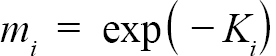
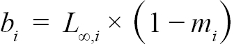
representing the slope and intercept of each individual’s Lt+1 vs Lt plot respectively, were obtained (with Ki and L∞,i representing the K and L∞ of individual i). Additionally, m = mean(mi) and b = mean(bi), representing the population slope and population intercept respectively, were calculated. Letting αi and βi represent the deviations of each mi from m and each bi from b, respectively, the equations for approximating population L∞ and K values are as follows (Hart and Chute, 2009a):
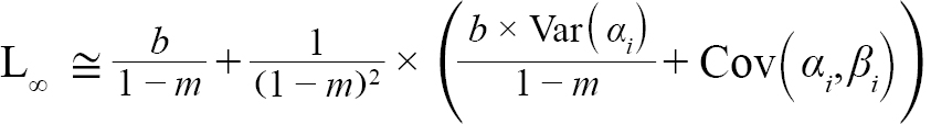 (4)
(4)
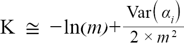 (5)
(5)
with Var(αi) and Cov(αi,βi), being the variance of αi and covariance of αi and βi, respectively. Additionally, the standard errors (σ) of L∞ and K were approximated as (Hart and Chute, 2009a):
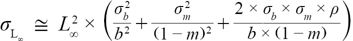 (6)
(6)
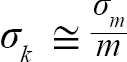 (7)
(7)
with σL∞, σK, σb, and σm representing the standard errors of L∞, K, b, and m respectively. All calculations were completed using R software (version 3.4.1). All R scripts used in modelling and analyses can be made available upon request.
Modelling Environmental Effects
L∞ and K cannot be associated with a particular year, only a location (they are constant throughout an individual scallop’s life). Thus, these values cannot be matched to any time-dependent environmental covariates. Because of these limitations, a different response variable had to be chosen for regression testing. The variable chosen was the change in length from one ring to the next: the growth over the course of a time-step in millimeters: Δmm. Because ASCs are sedentary after their spat stage (before 1 year old), each Δmm can be associated with a location (latitude and longitude), a time (year of growth), and by extension, abiotic variables associated with those locations and averaged over that year. The variables used in this study were bottom temperature (Figs. 3 and 4) and bottom salinity (Fig. 5). Additionally, because Δmm varies widely between age classes, separate regression tests were conducted for each, allowing for any age-specific environmental interactions to be explored.
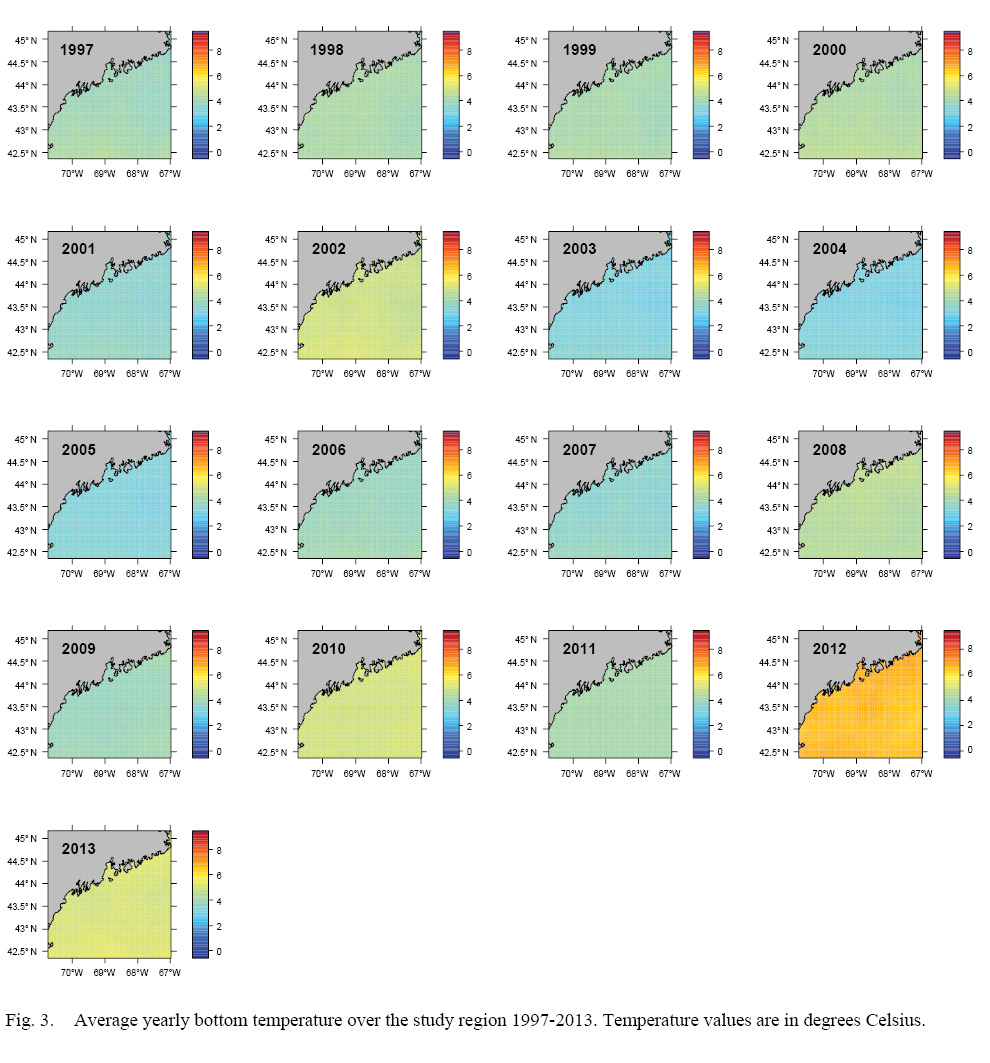
Fig. 3
Bottom temperature and bottom salinity data were obtained from University of Massachusetts (UMass) Dartmouth School for Marine Science and Technology (SMAST)’s Finite Volume Community Ocean Model (FVCOM). This geophysical model has been shown to have reliable performance in predicting bottom water parameters at fixed locations called stations, especially for well-stratified areas like the NGOM (Li et al., 2017). For each ASC, an average bottom temperature and salinity was obtained for each year of its growth. If the location of the tow was within ½ kilometer (km) of a FVCOM station, then the closest station was used to determine the abiotic conditions at the tow location. If no FVCOM station existed within ½ km radius, then the average of all FVCOM stations within a 1 km by 1 km grid centered on the tow location was used as a proxy.
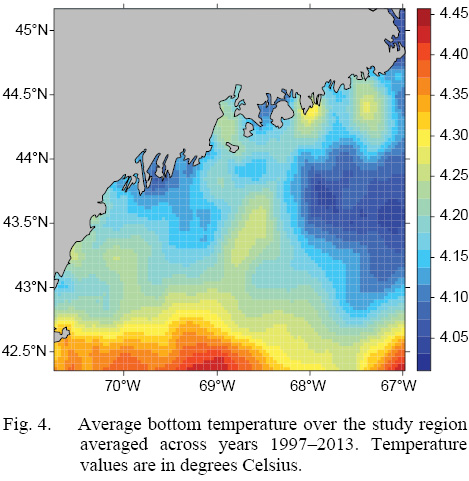
Fig. 4
Correlation coefficient calculation and variance inflation factor (VIF) tests were used to determine which combinations of predictor variables could be used together to have reliable regression output. Correlation coefficient values outside the range of (-0.5, 0.5) for a correlation coefficient meant those variables could not be used in the same test due to high collinearity. VIF values greater than 10 represent high multi-collinearity and do not allow for those variables to be used together in the same regression (O’brien 2007). These methods were used in tandem: correlation coefficients for all combinations of two factors were calculated and then VIF tests were conducted on all factor combinations used in regressions. This was done as to assume high robustness in factor selection for regression testing.
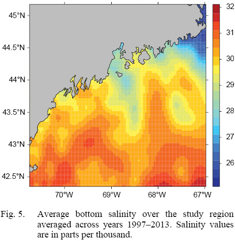
Fig. 5
Three different types of regression testing were conducted on each combination of factors that passed the two-step process above: linear regression (LR), boosted regression trees (BRT), and generalized additive models (GAMs). Model selection was based on root mean squared error (RMSE) and Akaike information criterion (AIC). Additionally, in an effort to further explore patterns in temporal trends, an additional six regression tests were run for each age class with year of growth as the only predictor variable only for ASCs from Cobscook Bay. The intent of these six models was to see if temporal trends could be more readily determinable if spatial differences were ignored.
Results
Spatial Differences in Growth Parameters L∞ and K
Final L∞ and K spatial values with associated standard errors are presented in Tables 1 and 2. L∞ was statistically different in the NGOM compared to Georges Bank (GB) and the Mid-Atlantic Bight (MAB) (One-way Anova test: F(2, 9030) = 654.54, p < 0.01, Tukey’s post hoc: all p < 0.01), with an apparent increasing trend in L∞ with increasing latitude (Table 1). K was statistically different in the NGOM compared to GB and the MAB (One-way Anova test: F(2, 9030) = 227.50, p < 0.01, Tukey’s post hoc: all p < 0.01), but no trend was apparent (Table 1). Data for GB scallops and MAB scallops were obtained from Truesdell (2014) and Hart and Chute (2009a).
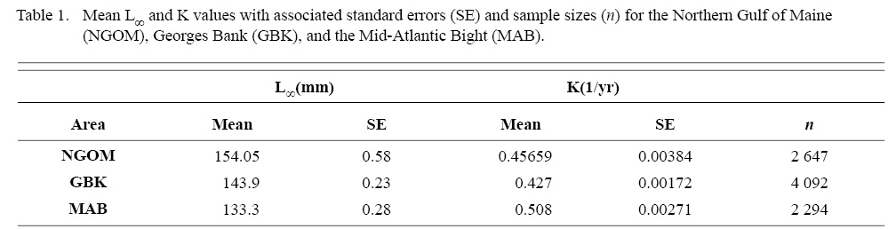
Table 1
Within the NGOM, L∞ was statistically different in all 4 management zones (One-way ANOVA test: F(3, 2643) = 146.02, p < 0.01, Tukey’s post hoc: all p < 0.01), with highest values in Zone 2 and lowest in Zone 3 (Table 2). K was statistically different across all three inshore zones, but Zone 4 was only statistically different from zones 1 and 3 (One-way ANOVA test: F(3, 2643) = 67.89, p < 0.01, Tukey’s post hoc: p < 0.01 for zone parings 1and2, 1and3, 1andoffshore, 2and3, and 3andoffshore, p > 0.05 for zone pairing 2andoffshore), with highest values in Zone 3 and lowest values in Zone 2 (Table 2). ASCs in Zone 1 appear to have the potential to grow to larger sizes than those in Zone 2, yet at a slower rate (Table 2). Cobscook Bay scallops (Zone 3) grow very rapidly, but do not reach the large sizes they do in the rest of the NGOM. Additionally, offshore (Zone 4) ASCs tend to grow at similar rates to scallops in Zone 1.
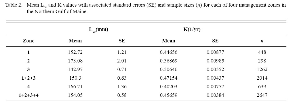
Table 2
Temporal Differences in Growth Parameters L∞ and K
Final L∞ and K temporal values with associated standard errors are presented in Table 3. L∞ was statistically different in most year classes than others, but with no discernable trend over the time series (One-way ANOVA test: F(12, 647) = 742.18, p < 0.01, Tukey’s post hoc results presented in Table 4). K was statistically different in some year classes than others, but with no discernable trend over the time series (One-way ANOVA test: F(12, 647) = 978.4075, p < 0.01, Tukey’s post hoc results presented in Table 5).
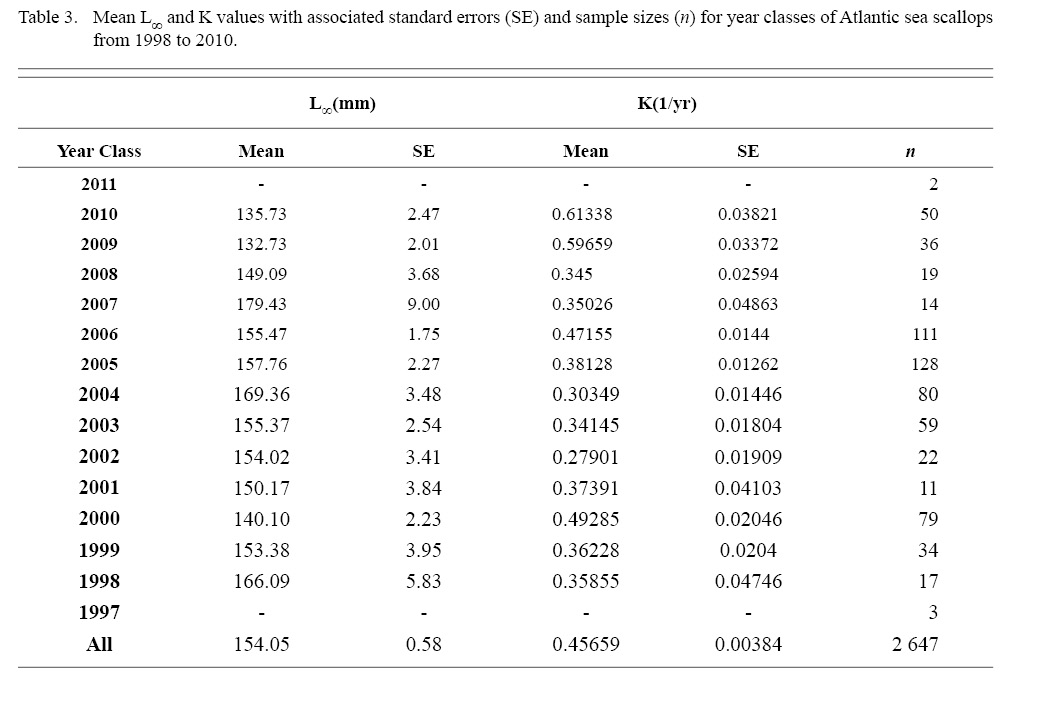
Table 3
Regression Model Selection
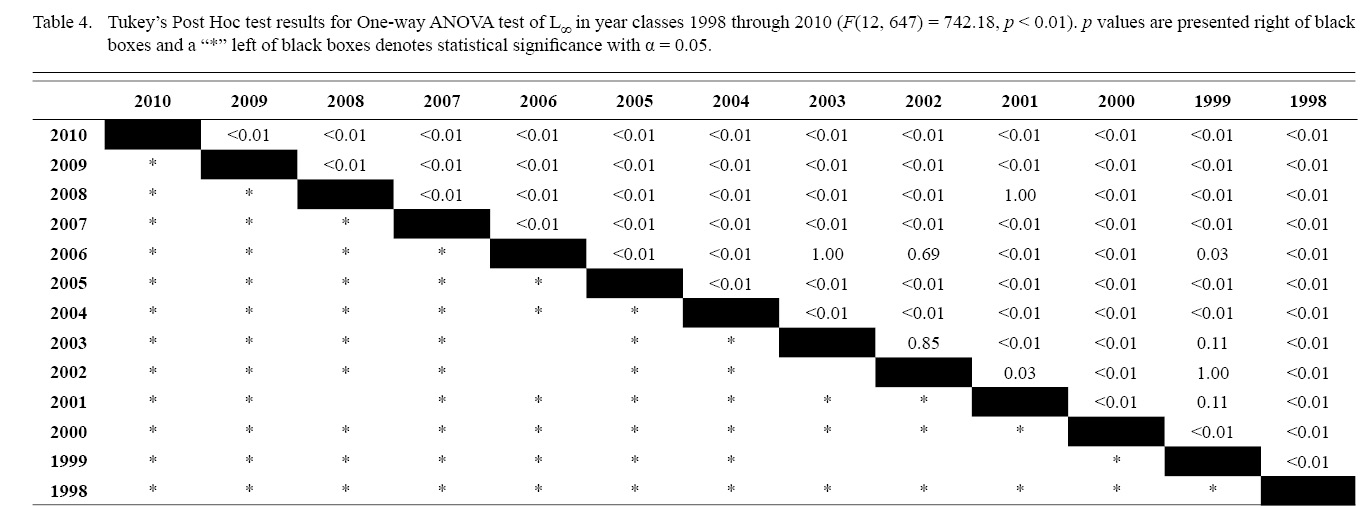
Table 4
Correlation coefficients and VIF values (Tables 6 and 7, respectively) allowed for 14 unique combinations of predictor variables. LR could not capture the appropriate trends in the data available. Due to very poor fit, this regression type was rejected. BRT and GAM both well outperformed LR, with BRT usually having lower RMSE (Table 9) and AIC values (Table 13) when compared to GAM (Table 8 for RMSE and Table 12 for AIC). However, GAMs allowed for the additional testing of spatial interaction terms more efficiently. Due to a general agreement in trends between BRT and GAM output, results from both types of regression testing are presented. Conclusions are made from both types of models.
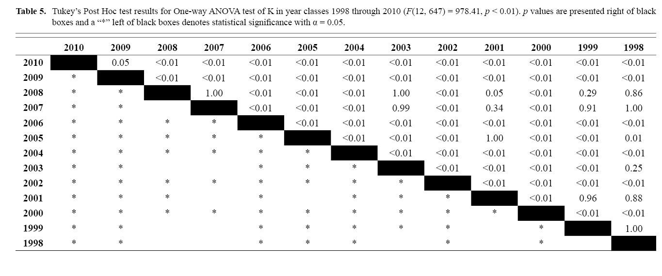
Table 5
Nineteen BRTs were run for each of six ASC age classes (Tables 9, 11, and 13): totaling 114 regression outputs. Twenty-two GAMs were run for each of six age classes (Table 8, 10, and 12): totaling 132 regression outputs. This discrepancy again is the testing of spatial interactions on single variables. An additional six GAMs were used to explore temporal trends in Cobscook Bay (see section 2.3). Neither GAMs nor BRTs are inherently and universally better than the other and model performance and fit depends on the data set (Martínez-Rincón et al., 2012). This accentuates the importance of testing multiple methodologies for modelling different data sets.
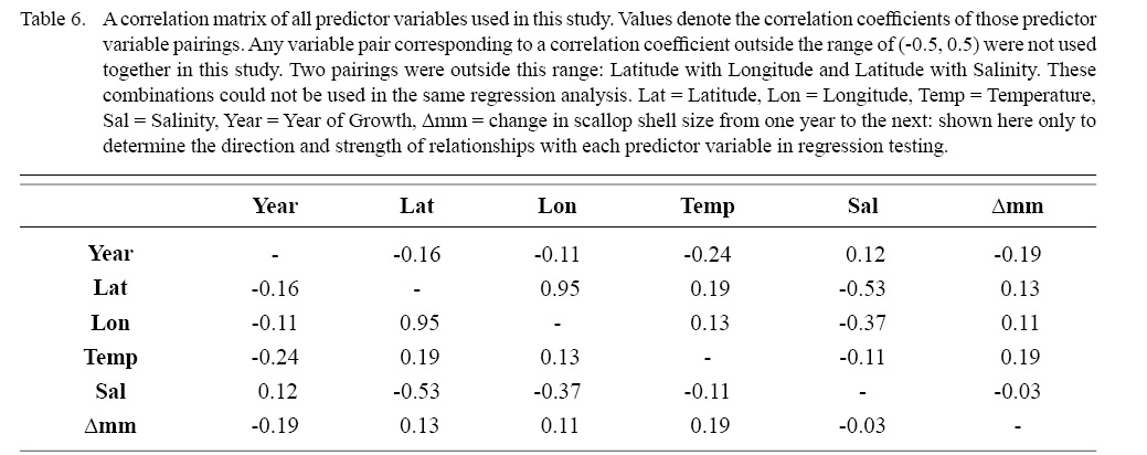
Table 6
Results of Regression Analyses
Deviances explained (DE) and AICs for all 114 BRTs in this study are presented in Tables 11 and 13, respectively. Highest DEs and lowest AICs usually coincided with each other (most being associated with the BRT with predictor variables year of growth, temperature, salinity, and longitude), with the exception of age classes 3–4 and 5–6. Even so, differences were not substantial. DEs and AICs for all 132 GAMs in this study are presented in Tables 10 and 12, respectively. Highest DEs and lowest AICs usually coincided with each other (most being associated with the GAM with predictor variables year of growth, temperature, salinity, and longitude), with the exception of age classes 2–3 and 6–7. Even so, differences were not substantial.
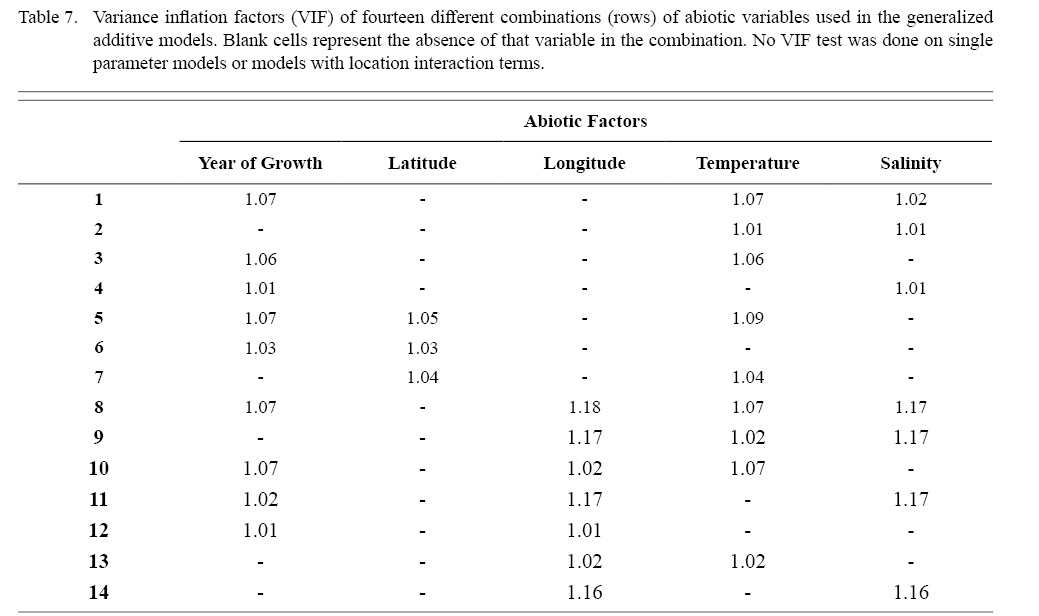
Table 7
DEs for BRTs were usually higher than those for GAMs. All DEs for GAMs were seemingly low; no DE surpassing 27%. The same was true for BRTs, with no DE surpassing 37%. Bottom temperature and salinity, therefore, are only capable of explaining at most 37% of the variance in ASC growth in the NGOM. Salinity alone explained more of the deviance in both types of models than temperature alone for all age classes, meaning ASCs in the NGOM appear to be affected more by salinity than by temperature. Concerning only the GAMs, predictor variables that included an interaction with location (both latitude and longitude) highly outperformed their counterparts; the same variable without a location interaction. This means that both temperature and salinity may affect ASC growth non-linearly over space and influences may vary by location. No clear trend was found to exist as a function of age class. The results of the correlation coefficient matrix (Table 6) seem to reveal that ∆mm has very weak positive relationships with each of the predictor variables except for year of growth and salinity, which both appear to be very weak negative relationships.
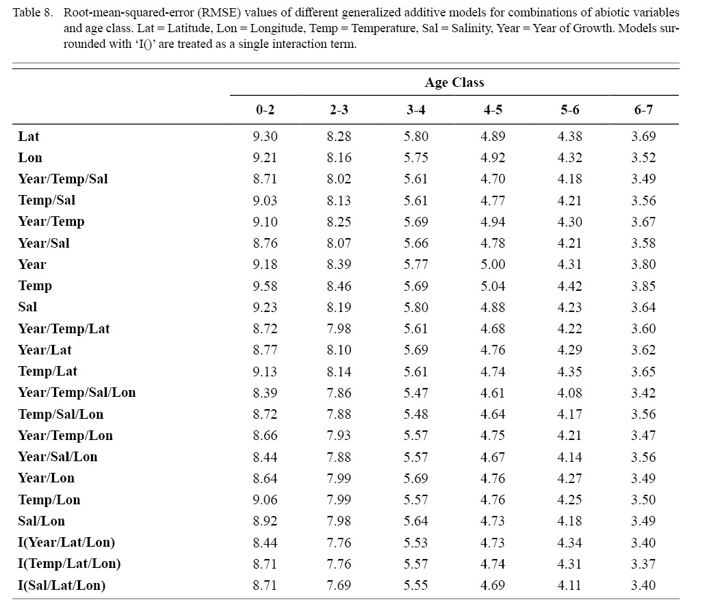
Table 8
The six regression analyses using data only from Cobscook Bay ASCs revealed results very similar to results pooled from the entire NGOM (Table 14), with the exception of the BRT for age class 3–4, whose DE was considerably high. In general, ignoring any spatial differences, it appears that year of growth alone does not sufficiently describe trends seen in scallop growth over time. This corroborates findings from section 3.2. It is important to note that of these analyses, only the first three age classes provided reliable results (Table 14). This was due to the often low number of older individuals (>4 years) found in Cobscook Bay over the time series.
Discussion
ASC in the NGOM appear to be growing to a larger size and growing at dissimilar rates when compared to populations in Georges Bank and the Mid-Atlantic Bight (Table 1; Truesdell, 2014; Hart and Chute, 2009a). A trend in growth coefficient L∞ seems to be occurring up the Atlantic coast, with ASCs of the Mid-Atlantic Bight having the lowest values and ASCs of the NGOM having the largest (Table 1). This is similar to findings from Truesdell (2014), which showed larger L∞ values for the NGOM region. Within the NGOM, ASC growth seems to vary spatially: varying between management zones (Table 2). This is again similar to findings by Truesdell (2014), but this study presents higher calculations of both L∞ and K for most regions. This could be due to the addition of new data since 2014 mostly concentrated inshore, where higher coefficients were observed.
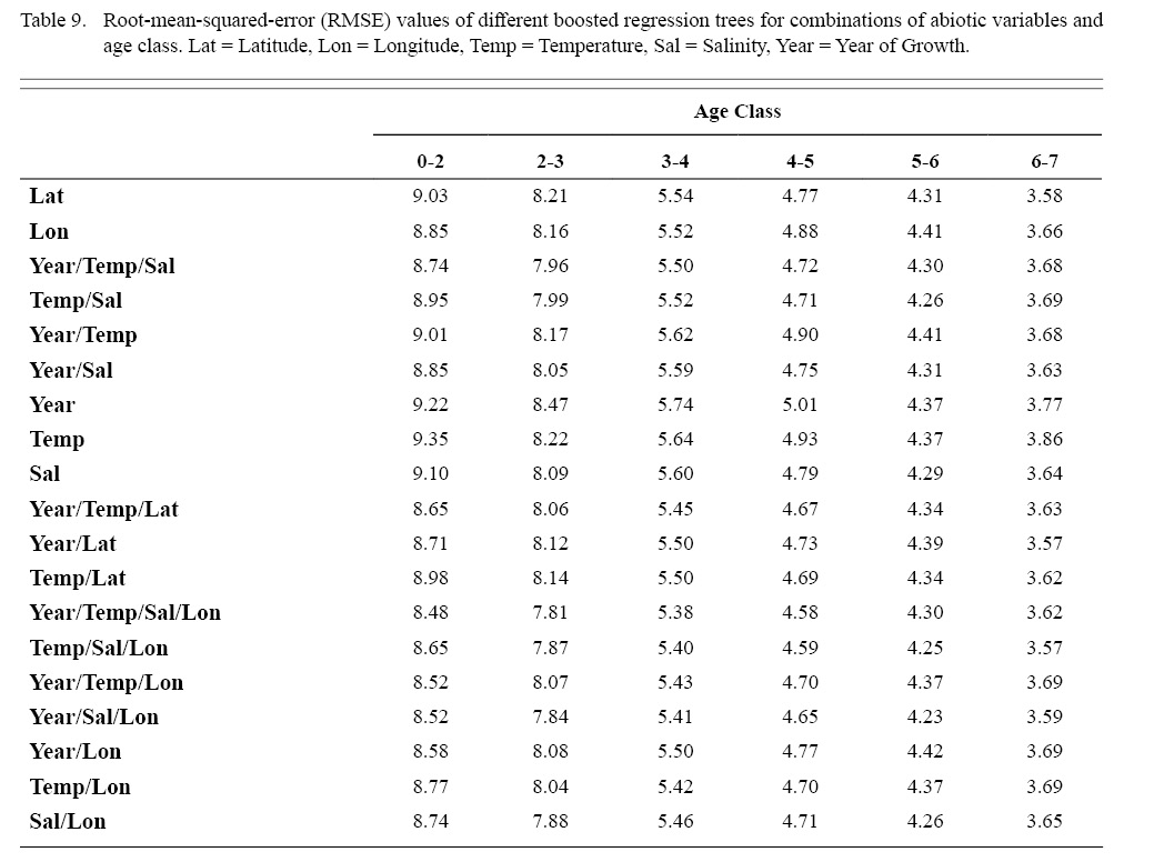
Table 9
This study expanded on work by Truesdell (2014), calculating growth coefficients for each year class. With low sample sizes questioning the reliability of some year classes, it doesn’t appear that ASC growth parameters are changing in a predictable way. They do seem to be fluctuating and ANOVA tests revealed those fluctuations result in year classes that are statistically different from one another. Due to the ever-changing location of MDMR tow stations in this project over the time series coupled with the low sample size per year class in this analysis, this fluctuation and by extent the statistical differences may not be what would be observed with larger sample sizes over the same time series. However, when spatial data were ignored in the Cobscook Bay subsample regression tests (which also have the highest density of samples of any region in this study), there was no more considerable influence of year of growth when compared to the original analyses with spatially pooled data over years.
These differences in growth over time do not match the change in the abiotic parameters observed in this study. Given that the regression analyses revealed that these parameters do have influence on ASC growth in the NGOM, it could be that pooling all data spatially does not allow for observation of these influences. Given that many studies have shown strong links between growth and temperature and salinity (Thouzeau et al., 1991; Stewart and Arnold, 1994; Hart and Chute, 2004), these effects may occur at finer spatial scales than what was used in this study. This highlights the need for more samples in the future so that finer spatial resolutions than what was utilized in this study can be explored.
The regression tests revealed that ASCs in the NGOM appear to be influenced by both temperature and salinity when abiotic data are not observed as spatial averages over time. However, these influences are relatively weak considering the deviance explained values associated with the tests. This highlights an important constriction of this study: abiotic data were temporally averaged in order to be associated with an increment of ASC growth. Future studies should look at abiotic ranges, anomalies, normality of distribution, and the like to infer more fine-scale temporal influences of these variables. Knowing this as a limitation, it can be assumed that the influence of temperature and salinity on ASC growth in the NGOM would be at least as strong as what was observed in this study, but has the potential to be stronger if abiotic data in a form other than yearly averages were utilized.
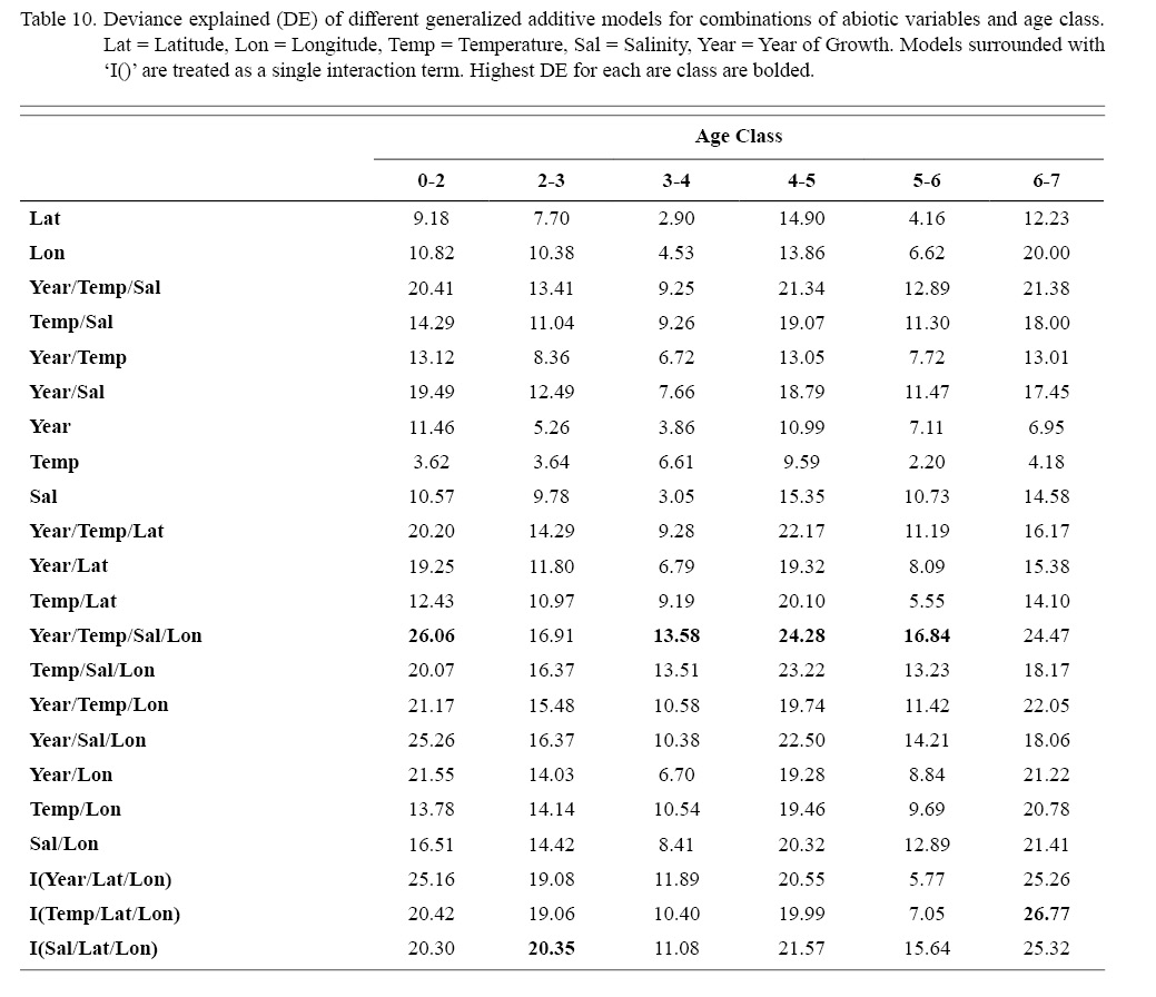
Table 10
Additionally, when temperature and salinity were supplied with an interaction term of location, the DE rises substantially. This could mean that ASCs in different areas of the Gulf of Maine respond differently to similar abiotic variables. This is most likely because these variables are acting in this study as a proxy for other variables known to heavily influence ASC growth such as phytoplankton density (Macdonald and Thompson, 1985a; Macdonald and Thompson, 1985b; Macdonald et al., 1987). Phytoplankton represent ASC food supply and mollusk growth has been shown to be highly correlated with phytoplankton density (Pilditch and Grant, 1999; Weiss et al., 2007). Phytoplankton density is a function of temperature, salinity, and other factors (Wagner et al., 2001; Friedland et al., 2015). The interaction term of location could be accounting for some of these other location-sensitive variables in the NGOM. This could also hinder the ability to determine direct abiotic-growth relationships if most influence is acting through a different force and these highly complex abiotic-growth relationships acting through proxy would be difficult for regression models to calculate. This accentuates the assumption that abiotic-growth influences were underestimated in this study. However, this study was aware of this connection when selecting the original model parameters. Given that the Gulf of Maine is changing rapidly in the face of climate change (Pershing et al., 2015), it was important to determine any direct relationships that ASC growth had to the abiotics directly affected by this change: temperature and salinity. This is why no model selection process took place based on AIC. This study was not meant to create a model for ASC growth, but to use multiple models to tease apart relationships.
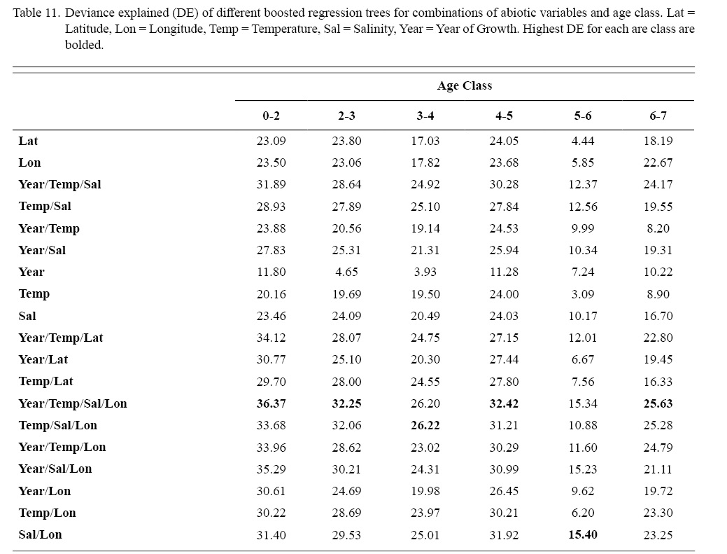
Table 11
Even though abiotic-growth relationships were relatively weak in this study, they were still present. These relationships have the potential to be affected in the coming years by climate change. Warming rates for the NGOM are suggested between 0.02˚C and 0.07˚C per year (Pershing et al., 2015) for sea-surface temperature, with bottom temperature experiencing this same trend (Pershing et al., 2015; Saba et al., 2016). Average yearly bottom temperature mean for all sample locations in this study area in recent years (2012–2016) averaged around 7.60˚C. These values are below optimal growth temperatures of 10.0˚C to 15.0˚C for ASC (Thouzeau et al., 1991; Hart and Chute, 2004), and well below the maximum temperature threshold of 21.0˚C (Hart and Chute, 2004). Bottom salinity is also expected to rise for the NGOM under climate change (Saba et al., 2016). Average yearly bottom salinity mean for all sample locations in this study area in recent years (2012–2016) averaged around 31.9‰. These values are below optimal growth salinity of full strength seawater: ~35‰ (Stewart and Arnold, 1994; Hart and Chute, 2004). With temperature and salinity in the NGOM both rising, and because of the relationships teased apart in this study, as well as support from previous research on optimal growth conditions (Thouzeau et al., 1991; Stewart and Arnold 1994; Hart and Chute, 2004), there is potential for ASCs to grow faster and/or larger. However, this conclusion is strictly based on direct and uniform relationships. Most studies focused on determining abiotic influence to ASC growth usually linking fluctuations directly to something like metabolic activity (Pilditch and Grant, 1999) and are done so in the lab. If conclusions from these studies state high influence of variables like temperature and salinity to growth, this may not be that accurate in a natural setting where these variables are acting both directly and through proxy. Because these variables are most likely acting both directly on ASC metabolism and indirectly through things such as food availability and can vary spatiotemporally, it can be difficult to infer the magnitude of the change in ASC growth given large changes in temperature and salinity.
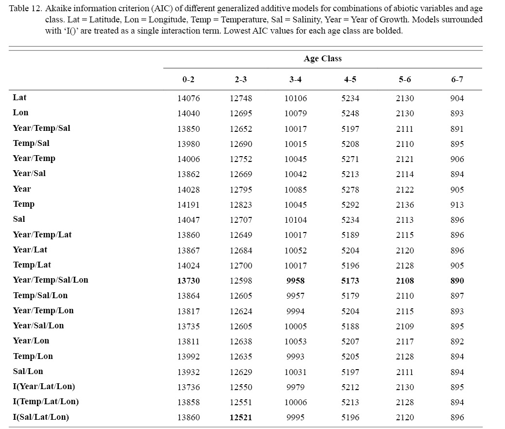
Table 12
Other ASC stock characteristics like abundance are more easily calculable from abiotic data through use of habitat suitability indices (HSIs). Torre et al. (2018) suggests that inshore habitats will become more suitable for ASCs in the NGOM as temperature and salinity rise. With suitable habitat predicted to rise and with a potential for increased growth, the NGOM may be able to support a higher intensity fishery in the future.
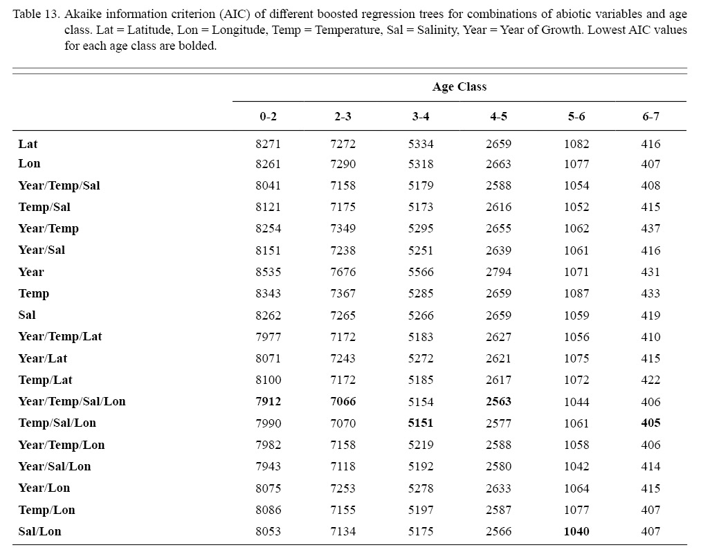
Table 13
There is need for more research concerning ASC life history and climate change to better understand their dynamics in the inshore NGOM. This study has shown the impact of abiotic variables on ASC growth to be weak yet present in this region. As suggested in other studies, biotic variables such as phytoplankton density, are posited to be more influential to ASC growth with abiotic variables influencing ASC growth directly and through this proxy of food availability. Future research should consider biotic variables as well as geospatial variables such as depth in an effort to better understand the NGOM ASC population dynamics.
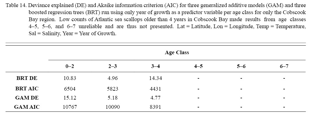
Table 14
Acknowledgements
We thank all the research assistants who help read the scallop ages. We additionally thank Dr. D. Hart and T. Chute of NOAA Northeast Fisheries Science Center and Dr. Sam Truesdell of MA Marine Fisheries for training in scallop aging. Lastly, we thank the Maine Department of Marine Resources and NOAA Fisheries for sample and data collection. The financial support of this study was provided by the Maine Department of Marine Resources and NOAA Scallop RSA Program. There is no conflict of interest declared in this article.
References
Chute, T., Wainright, S., and Hart, D. 2012. Timing of shell ring formation and patterns of shell growth in the sea scallop Placopecten magellanicus based on stable oxygen isotopes. Journal of Shellfish Research. 31: 649–662. https://doi.org/10.2983/035.031.0308
Côté, J., Himmelman, J., Claereboudt, M., and Bonardelli, J. 1993. Influence of density and depth on growth of juvenile sea scallops (Placopecten magellanicus) in suspended culture. Canadian Journal of Fisheries and Aquatic Sciences. 50: 1857–1869. https://doi.org/10.1139/f93-208
Durbin, E., Campbell, R., Casas, M., Ohman, M., Niehoff, B., Runge, J., and Wagner, M. 2003. Interannual variation in phytoplankton blooms and zooplankton productivity and abundance in the Gulf of Maine during winter. Marine Ecology Progress Series. 254: 81–100. https://doi.org/10.3354/meps254081
Fabens, A. 1965. Properties and fitting of the von Bertalanffy growth curve. Growth. 29: 265–289
Friedland, K., Leaf, R., Kane, J., Tommasi, D., Asch, R., Rebuck, N., Ji, R., Large, S., Stock, C., and Saba, V. 2015. Spring bloom dynamics and zooplankton biomass response on the US Northeast Continental Shelf. Continental Shelf Research. 102: 47–61. https://doi.org/10.1016/j.csr.2015.04.005
Harris, B., and Stokesbury, K. 2006. Shell growth of sea scallops (Placopecten magellanicus) in the southern and northern Great South Channel, USA. ICES Journal of Marine Science. 63: 811–821. https://doi.org/10.1016/j.icesjms.2006.02.003
Hart, D., and Chute, T. 2004. Sea scallop, Placopecten magellanicus, life history and habitat characteristics. NOAA Technical Memorandum NMFS-NE-189. 32 pp.
Hart, D., and Chute, T. 2009a. Estimating von Bertalanffy growth parameters from growth increment data using a linear mixed-effects model, with an application to the sea scallop Placopecten magellanicus. ICES Journal of Marine Science. 66: 2165–2175. https://doi.org/10.1093/icesjms/fsp188
Hart, D., and Chute, T. 2009b. Verification of Atlantic sea scallop (Placopecten magellanicus) shell growth rings by tracking cohorts in fishery closed areas. Canadian Journal of Fisheries and Aquatic Sciences. 66: 751–758. https://doi.org/10.1139/F09-033
Li, B., Tanaka, K., Chen, Y., Brady, D., and Thomas, A. 2017. Assessing the quality of bottom water temperatures from the Finite-Volume Community Ocean Model (FVCOM) in the Northwest Atlantic Shelf region. Journal of Marine Systems. 173: 21–30. https://doi.org/10.1016/j.jmarsys.2017.04.001
Marin, F., and Luquet, G. 2004. Molluscan Shell Proteins. Comptes Rendus Palevol. 3(6-7): 469–492. https://doi.org/10.1016/j.crpv.2004.07.009
MacDonald, B., and Thompson, R. 1985a. Influence of temperature and food availability on the ecological energetics of the giant scallop Placopecten magellanicus I: growth rates of shell and somatic tissue. Marine Ecology Progress Series. 25: 279–294. https://doi.org/10.3354/meps025279
MacDonald, B. and Thompson, R. 1985b. Influence of temperature and food availability on the ecological energetics of the giant scallop Placopecten magellanicus II: reproductive output and total production. Marine Ecology Progress Series. 25: 295–303. https://doi.org/10.3354/meps025295
Macdonald, B., Thompson, R., and Bayne, B. 1987. Influence of temperature and food availability on the ecological energetics of the giant scallop Placopecten magellanicus IV: reproductive effort, value and cost. Oecologia. 72: 550–556. https://doi.org/10.1007/BF00378981
Mann, R. and Rudders, D. 2019. Age structure and growth rate in the sea scallop Placopecten magellanicus. Virginia Institute of Marine Science, College of William and Mary.
Martínez-Rincón, R., Ortega-García, S., and Vaca-Rodríguez, J. 2012. Comparative performance of generalized additive models and boosted regression trees for statistical modeling of incidental catch of wahoo (Acanthocybium solandriEcological Modelling. 233: 20–25. https://doi.org/10.1016/j.ecolmodel.2012.03.006
Maunder, M. and Piner, K. 2015. Contemporary fisheries stock assessment: many issues still remain. ICES Journal of Marine Science. 72(1): 7–18. https://doi.org/10.1093/icesjms/fsu015
Mills, K., Pershing, A., Brown, C., Chen, Y., Chiang, F., Holland, D., Lehuta, S., Nye, J., Sun, J., Thomas, A., and Wahle, R. 2013. Fisheries Management in a Changing Climate: Lessons from the 2012 Ocean Heat Wave in the Northwest Atlantic. Oceanography. 26(2): 191–195. https://doi.org/10.5670/oceanog.2013.27
Northeast Fisheries Science Center (NEFSC). 2018. 65th Northeast Regional Stock Assessment Workshop (65th SAW) Assessment Summary Report. US Department Commerce, Northeast Fisheries Science Center Reference Document. 18–08; 38 pages. Available from: http://www.nefsc.noaa.gov/publications/
O’brien, R. 2007. A Caution Regarding Rules of Thumb for Variance Inflation Factors. Quality and Quantity. 41(5): 673–690. https://doi.org/10.1007/s11135-006-9018-6
Pershing, A., Alexander, M., Hernandez, C., Kerr, L., Le Bris, A., Mills, K., Nye, J., Record, N., Scannell, H., Scott, J., Sherwood, G., and Thomas, A. 2015. Slow adaptation in the face of rapid warming leads to collapse of the Gulf of Maine cod fishery. Science. 350(6262): 809–812. https://doi.org/10.1126/science.aac9819
Pilditch, C., and Grant, J. 1999. Effect of temperature fluctuations and food supply on the growth and metabolism of juvenile sea scallops (Placopecten magellanicus). Marine Biology. 134(2): 235–248. https://doi.org/10.1007/s002270050542
Rheuban, J., Doney, S., Cooley, S., and Hart, D. 2018. Projected impacts of future climate change, ocean acidification, and management on the US Atlantic sea scallop (Placopecten magellanicus) fishery. PLoS ONE. 13(9). https://doi.org/10.1371/journal.pone.0203536
Saba, V., Griffies, S., Anderson, W., Winton, M., Alexander, M., Delworth, T., Hare, J., Harrison, M., Rosati, A., Vecchi, G., and Zhang, R. 2016. Enhanced warming of the Northwest Atlantic Ocean under climate change. Journal of Geophysical Research: Oceans. 121: 118–132. https://doi.org/10.1002/2015JC011346
Stewart, P., and Arnold, S. 1994. Environmental requirements of the sea scallop (Placopecten magellanicus) in eastern Canada and its response to human impacts. Canadian Technical Report of Fisheries and Aquatic Sciences. 2005:1–36.
Thouzeau, G., Robert, G., and Smith, S. 1991. Spatial variability in distribution and growth of juvenile and adult sea scallops Placopecten magellanicus (Gmelin) on eastern Georges Bank (Northwest Atlantic). Marine Ecology Progress Series. 74: 205–218. https://doi.org/10.3354/meps074205
Truesdell, S. 2014. Distribution, Population Dynamics and Stock Assessment for the Atlantic Sea Scallop (Placopecten magellanicus) in the Northeast US [PhD Thesis]. University of Maine, Orono, Maine.
Wagner, M., Campbell, R., Boudreau, C., and Durbin, E. 2001. Nucleic acids and growth of Calinus finmarchicus in the laboratory under different food and temperature conditions. Marine Ecology Progress Series. 221: 185–197. https://doi.org/10.3354/meps221185
Wanamaker Jr, A., Kreutz, K., Schöne, B., Pettigrew, N., Borns, H., Introne, D., Belknap, D., Maasch, K., and Feindel, S. 2007. Coupled North Atlantic slope water forcing on Gulf of Maine temperatures over the past millennium. Climate Dynamics. 31(2-3): 183–194. https://doi.org/10.1007/s00382-007-0344-8
Weiss, M., Curran, P., Peterson, B., and Gobler, C. 2007. The influence of plankton composition and water quality on hard clam (Mercenaria mercenaria L.) populations across Long Island’s south shore lagoon estuaries (New York, USA). Journal of Experimental Marine Biology and Ecology. 345: 12–25. https://doi.org/10.1016/j.jembe.2006.12.025
: Hodgdon, C.T., Torre, M., and Chen, Y. 2020. Spatiotemporal variability in Atlantic sea scallop (
Placopecten magellanicus) growth in the Northern Gulf of Maine.
J. Northw. Atl. Fish. Sci.,
51: 15–31. https://doi.org/10.2960/J.v51.m729