A state-space stock assessment model for American plaice on the Grand Bank of Newfoundland

Download Citation Data

Citation to clipboard

Reference management software (Endnote, Mendeley, RefWords, Zotero & most other reference management software)

LaTex, BibDesk & other specific software

Introduction

American plaice (Hippoglossoides platessoideson the Grand Bank of Newfoundland (NAFO Divisions 3LNO) supported an important commercial fishery historically, accounting for over ten percent of the Canadian groundfish fishery in the 1950s (DFO, 2011). The population size declined rapidly in the 1980s due mostly to overfishing and, although there has been no directed commercial fishing since 1994, there has since been little improvement in the state of the population (see e.g. Wheeland, 2018). The lack of recovery has been attributed to overfishing, which has occurred mainly through bycatch in the yellowtail flounder, skate, redfish, and Greenland halibut fisheries (Shelton and Morgan, 2005). It has also been suggested that an increase in the natural mortality rate due to changing ocean temperatures may also be contributing to the lack of recovery (COSEWIC, 2009).

The current stock assessment model for Grand Bank American plaice is an ADAPT virtual population analysis (see e.g., Lassen and Medley, 2001) that was introduced in the late 1990s. This model is based on catch-at-age data that are derived in part from landings estimates and does not account for the considerable uncertainty about the landings data (Wheeland et al., 2018). Sources of uncertainty include landings recorded as “unspecified flounder” by some countries in the earliest years of available data (see e.g. Pitt, 1972) and an increase in foreign catch outside the 200 mile economic exclusive zone in the mid-80s (e.g. South Korea reporting “non-specified flounder”, Brodie, 1986).More recently, the lack of scientific observer data in the NAFO Regulatory Area has resulted in the need to estimate landings via various methods, including effort ratios and daily catch records (Dwyer et al., 2016). As a result, the landings data may be under-estimated and a stock assessment model that incorporates uncertainty in these data may therefore provide a better assessment.

Another issue that has been noted in the current assessment for American plaice are retrospective patterns, which are consistent directional changes in estimates of stock size as years of data are removed from the assessment model (Mohn, 1999). Retrospective patterns are caused by changes in the accuracy of the data over time and/or spatial and time-varying population processes that are unaccounted for or mis-specified in the model (see e.g. Legault, 2009). Systematic retrospective patterns can lead to poor management advice as important population processes (e.g. biomass and fishing mortality) may be over- or under-estimated and can result in unsustainable or sub-optimal harvesting advice (Szuwalski et al., 2017). To promote sustainable management advice for American plaice on the Grand Bank of Newfoundland, a stock assessment model that reduces or eliminates retrospective patterns is valuable. State-space stock assessment models are ideally suited for this purpose as they can include random errors in the underlying population dynamics model (i.e. for population abundance and fishing mortality rates) thereby accounting for underlying time-varying population processes that contribute to retrospective patterns. Additionally, state-space models allow for errors in the data (see e.g. Nielsen and Berg, 2014; Cadigan, 2015; Albertsenet al., 2016), which is an improvement to the current VPA that treats the catch-at-age data as known with negligible error. In this paper, we present a state-space stock assessment model for American plaice on the Grand Bank of Newfoundland that reduces the retrospective problem and allows for errors in the landings data.

Materials and Methods

There are two components to a state-space stock assessment model: the process model and the observation model. The process model describes how the state of the unobserved fish stock abundance and fishing mortality rates at a given time depend on previous states. The observation model describes how the survey and commercial data depend on the unobserved states (see e.g. Aeberhard et al., 2018).

American plaice Process Model

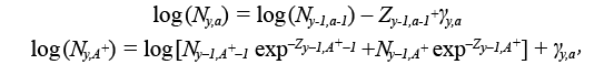
The model runs for the years y = 1960, ..., 2017 and for ages a = 1, ..., 15 +, where 15 + represents the oldest ages grouped together from ages 15 onwards, called the plus group (see Table 1 for model equations). For simplicity, we will refer to model ages a = 1, ..., A +, and years y = 1, ..., Y. The process model describes how the abundance at age a in year y (i.e. N y,a) and the fishing mortality, F y,a change over time. The N y,a for all ages and years are treated as random effects, with the cohort abundance model modelled as:

(1.1)

Table 1

where Z y,a = M y,a + F y,a is the total mortality rate given by the sum of the natural mortality rate, M y,a (i.e. all mortality unrelated to fishing) and F y,a. Here, M y,a is assumed to be known and fixed at 0.50 for ages 1–3, 0.30 for age 4 and 0.20 for all ages 5 and above, except during 1989 to 1996, where it is fixed at 0.53 for all ages 5 and above, as recommended by Morgan and Brodie (2001), 0.83 for ages 1–3 and 0.63 for age 4. This formulation for M y,a for ages 5 and greater is identical to the formulation for the most recent stock assessment model for Grand Bank American plaice. Here we also include ages 1–4, which are not currently used in the stock assessment VPA, with values for M at these ages selected through peer consultation. F y,ais set to zero for ages 1–4, as reported catch at these ages is considered negligible. The γ y,a are the process errors, assumed to be independent and normally distributed with variance σ pe 2  to be estimated. The numbers at the first age N y,1 are modelled as:

 (1.2)

where μ R y=μ R 1for y < 1993 and μ R y=μ R 2for y ≥ 1993, and the two mean recruitment parameters μ R 1, μ R 2 ∈ (− ∞, ∞) account for the large differences in recruitment between the two time periods and are fixed effect parameters to be estimated. The deviations from the mean recruitment δ R y are assumed to follow a normal distribution with AR(1) correlation across years, with the AR parameters σ 2 R  and ϕ R to be estimated across the entire time series, as we expect recruitment to be more alike in years that are closer together.

We assume that the fishing mortality rates increase with age, i.e.,

 for a= 7,..,15.  (1.3)

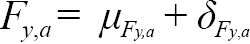
For ages 5 and 6, F y,a= μ F y,a + δ F y,a, where μ F y,a is the mean fishing mortality rate, a fixed effect parameter to be estimated. A separate μ F y,a is estimated for ages 5 and 6, for two blocks: 1960–1994 and 1995–2017 (i.e. four fixed effect μ F y,a parameters). The age blocking of the μ F y,a’s was chosen to reflect overall fishery selectivity patterns, and the year blocks were chosen to account for the closure of the commercial fishery in 1994. The δ F y,a are positive deviations from the fishing mortality rate at the previous age and are treated as random effects. The δ F y,aʼs are assumed to follow a normal distribution, with the deviations at the first age, δ F y,5, assumed to have AR(1) correlation across years with parameters σ F 5 2  , ϕ F 5to be estimated. We treat the δ F y,aʼs separately for age 5 fish as visual inspection of the catch-at-age data indicated that age 5 fish were not actively targeted in the earliest years of the fishery. The δ F y,aʼs at ages 6–15+ were treated as a correlated AR(1) process, separable across ages and years, with parameters σ F6 + 2  , ϕ F A6 +, ϕ F Y6 +to be estimated. We fit an AR(1) process across ages and years for age 6–15+ because fish that are closer in age and time are expected to have δ F y,athat are more similar than those that are further apart. The final formulation for the AR(1) parameters were determined via a model fitting process described in the exploratory process below.

Observation model

The observation model includes data from the commercial fishery and scientific research trawl surveys. There are two basic types of fishery information: total landed weight, and the size (length, weight) and age composition of the landings. Both these sources of information are used to derive annual fishery catch numbers-at-age. In the integrated assessment model philosophy, these data sources should enter into the assessment model fitting via separate observation models (i.e.one likelihood component for the age composition and one for the landings). We particularly want to focus our model estimation to include uncertainty in landings. Therefore, for pragmatic reasons, we used landings information (1960–2017) and the catch proportions-at-age (ages 5–15+ during 1960–2017) as independent data sources for model estimation. We only use commercial data from 1960 onwards as there was insufficient sampling before 1960. The current assessment model also does not use data prior to 1960. Age-based indices of stock abundance (i.e. numbers) are derived from the Canadian fall and spring research surveys in NAFO Divs. 3LNO (see Dwyer et al., 2014 for details) and the Spanish research survey in the portions of NAFO Divs. 3NO outside of the Canadian Exclusive Economic Zone (EEZ; González-Troncoso et al., 2017) were also used in model estimation. Indices were for ages 1–15+ for all surveys, for years 1990–2017 for the fall survey (2004 and 2014 omitted due to poor survey coverage), 1985–2016 for the spring survey (2006 and 2015 omitted due to poor survey coverage) and 1997–2016 for the Spanish survey.

Catch age composition data

We fit the age composition data using the continuation ratio logit (crl) transformation (see e.g. Cadigan, 2015; Berg and Kristensen, 2012; Agresti, 2003). A direct observation model for the matrix of observed catch proportions each year is complicated because of the constraints P oa ≥ 0 and ∑ P oa = 1. We use the crl which maps P a for a = 1, ..., A max into X a ∈ ( − ∞ , ∞) for a = 1, ..., A max − 1. The unconstrained crls are derived from the multiplicative logistic transformation,

 (1.4)

where A max is the plus group. Recall that there is no catch data for ages 1–4. The inverse transformation of (1.4) is:

 (1.5)

The crls for the observed catch proportions-at-age data (i.e. X oy,a) are calculated from (1.4) and the observation model we use is based on assuming the model residuals (X oy,a − X y,a) have a normal distribution with AR(1) correlation separable across ages and years with parameters ϕ C A, ϕ C Y, σ C y,a 2  to be estimated, as we expect the crl errors to be similar for fish that are closer in age and time. Various age and year formulations were explored for σ C y,a 2  and are described in the exploratory process below.

Landings data

Dwyer et al. (2016) reported uncertainties about the reliability of the landings data for Grand Bank American plaice. To account for this, we treat reported landings as a lower bound for true landings (i.e. not all catches are reported). We assume that there is an upper bound for landings that varies with the reliability of data (see Table 2 for details). We used a censored likelihood approach in which the bounds are treated as the only information about landings (see e.g. Hammond and Trenkel, 2005; Bousquet et al., 2010; Cadigan, 2015; Van Beveren et al., 2017). We assume the true landings could be accurately estimated with a CV of 5%. Let <Bly and Buy denote the lower and upper bounds and σ L = 0.05. The negative loglikelihood (nll) for the landings bounds data is:

Table 2

 (1.6)

where L 1, … , L Y are the model predicted landings. We fixed σ L at a small value to ensure that the estimates of landings are between the bounds for most years.

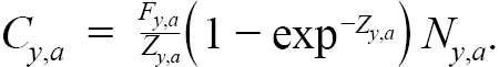
The Baranov catch equation is used to model commercial catch as a function of N, Fand Z,

 (1.7)

Model predicted catch proportion at age (P a = C a / ∑ a C a) were fit to observed proportions, as described in the previous section. Commercial average weights-at-age (W y,a) were calculated by Rivard’s method (Rivard, 1980) and are used to calculate model predicted landings each year, L y = ∑ a W y,a C y,a.

Survey data

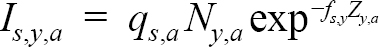
The model-predicted catch for survey s is:

 (1.8)

where f represents the fraction of the year the survey takes place (0.460 for the Canadian spring and Spanish surveys and 0.875 for the Canadian fall survey). As in our treatment of the fishing mortality rates, we model the survey catchabilities, q s,a, as increasing with age for each survey:

Here, the δ q s,a are positive deviations from the q s,ain the previous year and are treated as fixed effects. We note that the δ q s,a are always positive to ensure that the q’s increase with age and are treated as fixed effects since they are part of the observation equation and not the unobserved population process. For age 1 fish, the q s,a parameters are freely estimated, with no added deviation. In 1995 the trawl used in the Canadian surveys changed from the Engel to the Campelen (see e.g. Dwyer et. al., 2016). Although Engel catch data were adjusted based on information from comparative fishing to match the Campelen catches, in our model ages 1–4 are given a separate q for each gear period due to issues in conversion of survey catches at these ages (Dwyer et. al., 2016). The indices are assumed to follow a normal distribution, with mean I s,y,a and standard deviation σ s,a = cv s,a ∙ I s,y,a, where CV s represents a separate coefficient of variation (CV) parameter for each survey, to be estimated. Various age formulations for each survey CV were explored and are detailed in the exploratory process below. We treated each survey as from an AR(1) process across ages with independent parameters ϕ s to be estimated. A constant CV variance model for I is approximately the same as assuming log(I) has constant variance; however, an advantage of our approach is that we can use observed zero indices directly in the model whereas in other assessment packages these index zeros are typically excluded which is not appropriate when there are many zeros which occur non-randomly over time.

Estimation

The fixed-effects parameters to estimate (i.e. θ) are listed in Table 3. The unobserved states (i.e. δ F y,a, N y,a) are integrated out of the joint likelihood function and the estimation of θ is based on maximizing the marginal likelihood L(θ):

 (1.9)

Table 3

where Ψ is the vector of all random effects, f θ(D|Ψ) is the joint probability density function of the data (D; commercial landings, catch proportions at-age, commercial average weights-at-age, and Canadian fall, Canadian spring and Spanish survey indices) and g θ(Ψ)is the joint probability density function for the random effects. The TMB (Kristensen et al., 2016) package in R is used to integrate the marginal likelihood (1.9), which is performed via the Laplace approximation (see Skaug and Fournier, 2006 for details). The nlminb package in R is used to minimize the negative log likelihood function provided by TMB.

The final model formulation was determined via a thorough exploratory process. The overall goal of the exploratory process was to determine the best model formulation for the survey CVs, the crl σ C y,a 2  (sds) and the q age-aggregating (detailed below). The Bayesian information criterion (BIC) was used in model selection since BIC penalizes more heavily for extra parameters when the sample size is large. Previous work has shown that the correlation parameters can be difficult to estimate reliably (see, e.g., Johnson et al., 2016; Xu et al., 2019), thus for our exploratory process, we conducted four exploratory runs with fixed AR(1) parameters: S1) ϕ s freely estimated for each survey, all ϕ F= 0.90, ϕ C A= 0.9, ϕ C Y= 0.75; S2) ϕ s freely estimated for each survey, all ϕ F= 0.90, ϕ C A= 0.9, ϕ C Y= 0; S3) all ϕ s, ϕ F, ϕ C = 0.50; S4) all ϕ s, ϕ F,  ϕ C = 0. In all cases, the exploratory process began with the simplest model: with one sd parameter estimated for the crls, and one CV parameter per survey <(see Table 3) and followed the 6 steps below. Within each step, the model was refit for each assumption (e.g. in step 1 the model was refit 10 times, for q age-aggregating 5,..,14):

1) q age-aggregating: for each age 5,..,14 fix survey δ + q s,a = 0 for all subsequent ages (e.g. q5+ is one run with δ + q s,a fixed at 0 for ages 6+). q age-aggregating selected from run with lowest BIC1.

2) CV combinations: for each survey using q age-aggregating from 1) fit all combinations (pooled and unpooled; see Supplementary Materials 1 for details) of CV ages while keeping one CV parameter for other two surveys. Survey CV formulations for each survey selected from run with lowest BIC.

3) re-check q: with survey CVs from 2), re-run 1) to check that q age-aggregation is the same as in 1)

4) crl sd ages: with survey CVs from 2) and q from 1), fit all combinations of crl sd ages. crl sd age formulation selected from run with lowest BIC.

5) crl sd years: with q from 1), survey CVs from 2), and crl sd ages from 4), fit two scenarios:

a. pre/post moratorium split: fit a separate age sd parameter pre/post moratorium for year split start ∈ (1990, 1999)

b. moratorium gap: fit one separate sd parameter (no age splitting) for 10-year mortarium gap for year gap start ∈ (1990, 1999).

crl sd year formulation selected from run with lowest BIC from both a and b

6) re-check q: with survey CVs from 2), crl sd ages and years from 4–5, re-do 1) to check that q age-aggregation is the same as in 1)

The best fitting model was selected from step 6 for each of the four runs (i.e. one best fitting model for runs S1-S4 selected via lowest BIC from step 6) and model fit compared across all four via a detailed examination of model residuals and BIC. Evidence of patterns in residuals (i.e. blocks of ages and years having residuals of the same sign, and whether or not overall residual variability matches assumption) was used to evaluate potential model mis-specification. The survey and continuation ratio logit residuals, which are correlated in our observation models, were standardized using the Choleski factorization of their estimated covariance matrix. We did not use the one-step ahead residual method (see e.g. Thygesen et al., 2017) because it does not allow for correlations in the observations. A final model was selected from the four S1–S4 best fitting runs (i.e. via BIC and residual fits) and in the final step, two extra runs were fit; one with all ϕ F parameters freely estimated and all ϕ C fixed and one with all AR(1) parameters freely estimated (O2). These two runs were compared to the run with the fixed AR(1) parameters (O1), and a final model selected from the three. In all subsequent text, SSM will refer to the final model.

The SSM fit was also assessed through retrospective model fitting for the years 2011–2017. Each retrospective model fit used one less year of data (i.e. model for year 2011 used data up to 2011) and predicted abundance, biomass, spawning stock biomass and average F’s were examined for systematic patterns and the severity of retrospective pattern was assessed using Mohn’s rho (see Mohn, 1999). Ideally, no discernable directional patterns will be present in the retrospective plots.

Biomass-at-age was calculated by multiplying predicted numbers at age (i.e. N y,a) and stock weights-at-age, which were estimated externally via a spatiotemporal biphasic Von Bertalanffy growth model (see Kumar et al., 2020). Length and age data are collected for American plaice from research survey vessels using a length-stratified age sampling design and Perreaultet al. (2019) showed that ignoring this sampling design can lead to biased growth model parameter estimates. Kumar et al.’s method (2020) accounted for the length-stratified age sampling design. The 3LNO stock weights were combined for each division by weighting the values for each division by the average abundance index at age during 1975–2017. Stock weights prior to 1975 were fixed at the mean values for 1975–77. Estimates of maturity-at-age were taken from Wheeland et al.(2018).

Simulation and sensitivity testing

A full simulation study is beyond the scope of this paper; however, we conducted a simple self-simulation test and jittered start on the SSM to examine the reliability of the model estimates see e.g. Cadigan, 2015; Nielsen and Berg, 2014). The self-simulation test randomly generates survey indices and continuation ratio logit catch proportions from the model predictions and assumed distributions detailed above. Process errors and other random effects are treated as fixed when generating the data and the model is re-fitted to the simulated data. This process is repeated 1000 times and estimates of SSB, average fishing mortality rates (ages 9–14), recruitment, variance and autocorrelation parameters are stored. We calculated the relative difference of the estimates for each year (i.e. (simulation SSBydata-based SSBy)/ data-based SSBy) for comparison.

The jittered start test re-fits the model with random noise added to the starting parameter values, generated from N(0,0.25 ∙  ˆ μ ), where  ˆ μ  is the model predicted parameter of interest. The model is re-optimized 100 times and the negative log-likelihood is stored for each iteration. Ideally, we expect an identical model fit from the jittered starting parameter values.

We also examined the model sensitivity to our assumptions about M and catch bounds. A profile likelihood was constructed for a range of M a,yʼs; that is, M a,y = M + ΔM,  where M is the SSM M model formulation and ΔM ∈ ( − 0.1, 0.35). We also re-fit the model with upper catch bounds fixed at half the original model formulation upper bounds (M2) and with the upper catch bounds fixed (M3) at 1% of the reported bounds (i.e. “fixed landings”). Model fit for the catch bounds was assessed using BIC and an examination of the retrospective plots.

Results

For brevity, we provide a summary table of the exploratory process that describes the final model from each run (Table 4); additionally, only the full exploratory process results from the best fitting run (S2) are given in see Supplementary Materials 1 (SM1) and discussed. For exploratory step 1 (run S2), the model with an age-aggregation of 7+ (δ + q s,a = 0 for ages 8+) had the lowest AIC and this was selected as the age-aggregation for step 2 (see footnote 2 for details and SM1 Table 1). Overall, the BIC for the fall model fits ranged between approximately 9970 and 9890, 9940 and 9860 for the spring survey and 9970 and 9900 for the Spanish survey, indicating the grouping of the Spanish survey coefficient of variations (CVs) provided the least improvement in model fit (SM1 Tables 2–5). This is not surprising since the data for the Spanish survey do not cover the entire 3LNO region and are not as informative as the fall and spring surveys (see, e.g. Wheeland et al. 2018 for more details). Rechecking the q age-aggregation in Step 3 confirmed that the age-aggregation of 7+ provided the lowest AIC and BIC with the new survey CV formulations (SM1 Table 6). The continuation ratio logit (crl) age exploratory runs in Step 4 had BICs that ranged from approximately 9600 to 9570, and the age aggregation of (5–6)(7–11)(12–14) was selected as the final crl sd age formulation (SM1 Table 7). For Steps 5a and 5b, the BICs ranged from approximately 9560 to 9480 (SM1 Table 8). Rechecking the q’s in Step 6 confirmed that the age-aggregation of 7+ provided the lowest AIC and BIC with the new survey CV and crl sd formulations (SM1 Table 9). The AIC and BIC from Step 1 with a q age-aggregation of 7+ were 9690 and 9922 in comparison to the Step 6 run that were 9194 and 9481 respectively, indicating a substantial improvement in model fit.

Table 4

In all four exploratory model scenarios, q7+ was the best formulation for the survey catchabilities (q; Table 4). Overall, the survey CV formulations were similar for all four model formulations. For example, for the fall survey, models S1–S3 provided identical formulations, with S4 (all AR(1) parameters fixed to zero) providing a better fit with an extra CV parameter for ages (2–4). Both the spring and Spanish CV formulations were similar for all four runs, providing the best fit with separate parameters at the oldest and youngest ages. In all formulations, the best fit for the crl sd parameters had a separate variance parameter from 1990–1999, with various formulations for the age groupings. For example, S1 provided the best fit with separate sd parameters for ages 5–7,14, and pooled for ages (8–13), whereas S4 pooled the sd parameters for ages (5–11) and (12–14). Overall, S2 had the lowest BIC, and had the best residual fits for both the surveys and the crls (see Supplementary Materials 2), and we selected this model as the best fitting model. For the final exploratory step (i.e., one run with all ϕ F parameters freely estimated and all ϕ C fixed and one run with all AR(1) parameters freely estimated), the lowest BIC was for the model with all but the crl AR(1) parameters freely estimated (SSM; Table 5), and this was selected as the final state space model.

Table 5

The SSM fit the data well with no patterns in the survey or continuation ratio logit residual plots (see Supplementary Materials 3). In 2017, recruitment, abundance and spawning stock biomass (SSB) were estimated near the lowest historical levels (Fig. 1). The model predicted landings were estimated within the upper and lower bounds, with the predicted landings closest to the upper bound in the early 80s, and again in 2010 (Fig. 2) and closest to the lower bound in the early 1990s. At ages 1–4, the catchability pattern (Fig. 3) for the fall and spring surveys was lower for the Engels than the Campelen trawl. The differences were most pronounced for ages three and four, with the catchability estimates for the Campelen trawl almost twice as large as for the Engels trawl. For ages 1–5, the process errors (Fig. 4) were close to zero until the mid-nineties. Overall, there were no noticeable trends in the process errors at the older ages. Mohn’s rho for the full retrospective run (Fig. 5) was 0.30 for abundance and -0.19 for recruitment. In comparison to the most recent stock assessment model for Grand Bank American plaice (which we refer to as the VPA), the SSM had a lower Mohn’s rho for SSB at 0.43 compared to 0.69 for the VPA (Fig. 6). Mohn’s rho for aveF for the SSM was almost half the VPA Mohn’s rho, at -0.27 for the SSM and -0.45 for the VPA.

Fig. 1

The overall trends in SSB and aveF were similar for the SSM and the VPA (Fig. 7). Noticeable differences included the SSM predictions of historical SSB (i.e. years 1960–1972) that were larger (but with high uncertainty) than the historical SSB predictions from the VPA. The VPA model also predicted a higher average fishing mortality rate in the early 1990s, at approximately 1.1, with the SSM prediction at approximately 0.80 for the same period.

Fig. 2

The self-simulation study lower 2.5% and upper 97.5% intervals for both SSB and aveF covered zero until the mid-1990s,(Fig. 8), indicating that the simulated samples produced estimates that were similar to the SSM estimates in those years. In the earliest years (1960–1972), the median of relative differences for aveF was mostly positive, with the converse for SSB. After 1990, there was a consistent positive bias in aveF and a negative bias in SSB, except in the final years, where aveF was underestimated and SSB overestimated. The boxplots of parameter estimates (Fig. 9) showed that the largest range were for estimated μ F 5_Pre1995. TMB has an option (see Thorson and Kristensen, 2016) to reduce bias in nonlinear random effects models, and we implemented this method in a self-simulation run as a potential fix to the bias in our self-simulation study (see M4; Table 5). The bias across the entire time series for both SSB and aveF was much larger with the bias-correction turned on (see Supplementary Materials 4) than without. The jittered-start test did not converge for 5% of the simulations, with 100% of the converged models producing negative log-likelihoods that were identical to the original formulation.

Fig. 3

The minimum negative log-likelihood from the M profile likelihood plot was 4472, with an associated Δ M of 0.30 (Fig. 10). For this model fit, the average fishing mortality rate in 2017 was estimated at 0.01 with SSB in 2017 at 100.83 hundred thousand tons. Results from the sensitivity tests (Table 5) showed that the SSM had a lower BIC than the runs that halved the catch bounds (M2) and “fixed” the landings (M3). This is expected because more narrow catch bounds restrict the flexibility of the model. Mohn’s rho for both M1 and M2 for aveF were slightly larger than the Mohn’s rho from the SSM at -0.29 (Fig. 11). Similarly, Mohn’s rho for M1 and M2 for SSB were slightly larger than for the SSM at 0.39.

Discussion

Overall, our state-space model (SSM) that accounted for uncertainties in the landings data and allowed for process errors fit the data well, with no obvious patterns in the survey and continuation ratio logit residual plots (see Supplementary Materials 3). The retrospective patterns were reduced for spawning stock biomass (SSB) and greatly reduced for average fishing mortality for ages 9–14 (aveF) compared to the most recent stock assessment model (VPA).

The M profile plot provided the best fit when M was increased by 0.30, suggesting that the values we used for M’s may be too low. Previous research found evidence that M’s during 1989 to 1996 (Morgan and Brodie, 2001) had increased to 0.53 and the current VPA model and our SSM include this increase. However, since the closure of the commercial fishery, estimates of total mortality rates have remained high for some periods (e.g. Fig. 7 for years 2000–2006), and this may suggest that M is higher than 0.20 in recent years. This is supported by preliminary work that suggests that M has increased since the mid-1990s (COSEWIC, 2009; Morgan et al., 2011). The lack of recovery of the stock has largely been attributed to overfishing, however the mis-specification of M not only in the SSM but in historical assessment models could be over-estimating the relative impact of F. Thus, although a thorough study of M is beyond the scope of this paper, research that improves our understanding of M for this species should be of high priority as we may be fixing M within the model to be lower than is reasonable and subsequently over-stating the contribution of fishing mortality to the lack of recovery of the stock.

Fig. 4

Mohn’s rho from the SSM retrospective analyses for both aveF and SSB were closer to zero than Mohn’s rho from the VPA retrospective analysis, which is a key improvement compared to the current assessment model. Including process error in the population dynamics model helped account for underlying time-varying population processes (e.g. M) that were not accounted for in the VPA, thereby reducing retrospective patterns. There is still evidence of slight retrospective patterns, and this may be caused by underlying spatial or time-varying processes that are mis-specified in the observation model since process errors can only account for misspecifications in the process equations.

Fig. 5

The estimate for survey catchabilityq is defined as the value required to scale swept-area abundance to the population abundance (see e.g. Dickson, 1993; Fraser et al., 2007). An estimate of q less than one implies that fewer fish are caught than occupied the area of the trawl, and a value greater than one implies that more fish are caught than occupied the area. Bryan et al. (2014) found evidence of herding behavior in over 90% of observed flatfish in the presence of survey trawls and this herding underestimates the width used in area swept calculations and can result in q estimates that are greater than one. Therefore, larger q estimates are not unrealistic for American plaice; however, the q estimates from the SSM are very large, with the maximum at 6.7. The maximum q estimate from the SSM is however much smaller than the maximum q estimated from the VPA at 13.62 (Table 26, Wheeland et al. 2018). Additional research is required to better understand why the stock assessment model estimates are so high.

Fig. 6

A difference to note between the SSM and the VPA is that the SSM assumes that the survey indices have a normal distribution with a constant coefficient of variation (CV) whereas the VPA assumes that the log of the survey indices have a lognormal distribution. The lognormal distribution does not allow for zeros in the survey data; however, this assumption may not be appropriate when there are many zeros in the data or when zeros are “true” zeros (i.e.no fish available to be caught). The assumption of normality with a constant CV avoids the problem of dropping zeros altogether. However, the normal distribution assumption supports negative indices which are infeasible. A solution to this problem is to use a truncated normal distribution in place of the normal distribution (e.g. Albertsen et al., 2016). However, a normal distribution with constant CV is virtually identical to a truncated normal distribution when the CV is small. Consider two random variables (e.g.Xand Y) that both have mean μ and a constant coefficient of variation, τ = σ / μ. If X~N(μ, σ = τμ) and Y~TN(μ, σ = τμ; Y > 0) has a truncated normal distribution then their density functions differ by a multiplicative constant that only depends on τ and does not depend on μ. The constant is ∫ 0 ∞ φ(z − 1 _ τ ) dz where φ(∙) is the density function for Z~N(0,1). The constant is close to 1 for τ < 0.5. Hence, for our model, using the truncated normal distribution instead of the normal distribution will only affect estimation through differences in the weighting of survey indices with differentτ’s, especially when τ ≫ 0.5. For our SSM we only have large τ’s for the Spanish survey and ages 1–2 for the Canadian surveys, thus in our case there should be little difference in model fit for the truncated normal vs the normal. However, although the approaches are theoretically similar, future research is needed to compare the performance of the three methods.

Fig. 7

Fitting the age composition and landings data separately is in line with the integrated model philosophy, but our treatment of stock and catch weights is not. Ideally, each source of data should enter independently into the likelihood equation; however, the stock and catch weights at age data for American plaice are collected in complex length-stratified sampling designs and how to model these likelihoods is difficult and beyond the scope of this paper. In the future, state-space stock assessment models will ideally fit to the raw data (e.g., maturity at age, weights at age) and this will require complex stock assessment models that can account for the spatial nature of the stock assessment data.

Fig. 8

The self-simulation study lower 2.5% and upper 97.5% did not cover zero for years 2006–2010 and again in 2013–2015. This bias was also present in models O1 (fixing all crl and F AR(1) parameters) and O2 (freely estimating all AR(1) parameters; (see Supplementary Materials 4). In a self-test simulation the model is specified exactly so stock size estimation bias cannot be the result of model misspecification, but rather it must be related to estimation bias and possibly related to nonlinear modelling of random effects. Our self-simulation run that implemented the TMB bias correction option had larger bias than the SSM self-simulation run without (see Supplementary Materials 4), which provides evidence that the bias is related to estimation bias. Also, preliminary research that fit the SSM with an increase in M (both across the entire time series, and another run increasing M only in the later years) did not produce the self-simulation bias in SSB and aveF in these later years (see Supplementary Materials 4). Hence, it seems that the bias is related to the particular settings of the model, and perhaps the magnitude of variance parameter estimates, and this requires additional research to better understand this type of bias.

Fig. 9

Although M profile plots are useful in providing a general picture of the role of the M assumption, it is also useful to examine which data sources are more informative about M, and Lee et al. (2011) suggested that informative length or age composition data is needed to reliably estimate M. Data-specific M profiles are commonly produced by more traditional stock assessment models without random effects and process error (e.g.SS3; Methot and Wetzel, 2013) but in a state-space stock assessment model it is not straight-forward how to do this because the integrated log-likelihood cannot be split into a sum of log-likelihoods due to various data sources and other model assumptions. Further development of diagnostics designed to detect M misspecification (e.g.Cadigan and Farrell, 2002) also seems useful.

Fig. 10

While overall trends in stock trajectory are similar, our new SSM is an improvement to the current stock assessment model that is used to inform the management of American plaice on the Grand Bank of Newfoundland as it allows for errors in the landings data and reduces the retrospective patterns. Additionally, the thoroughness of our model selection process has the potential to increase the confidence in the selected final model and thereby in the assessment output that is being provided to fisheries managers. Our results also suggest that the current values used for natural mortality rates may be too low as our diagnostic model fitting found the best model fit when M was increased by 0.30. This is an important note not only for American plaice, but for all stocks that are managed under the assumption of a fixed M. We suggest that M profile plots (and/or alternative diagnostics) should be routinely provided to facilitate a better understanding of model behavior for various assumptions about M. This can provide motivation for research into more realistic values of M for future stock assessment models. Overall, this model is a valuable first step in improving our understanding of the stock of American plaice on the Grand Bank of Newfoundland as the flexibility of state-space models are an ideal foundation to build more realistic models.

Fig. 11

Acknowledgements

Research funding was provided by the Ocean Frontier Institute, through an award from the Canada First Research Excellence Fund. Research funding to NC was also provided by the Ocean Choice International Industry Research Chair program at the Marine Institute of Memorial University of Newfoundland. Funding to AP was also provided by a Natural Sciences and Engineering Research Council of Canada Master’s Graduate Scholarship. Many thanks are also extended to Dr. Anders Nielsen, Danish Technical University, for advice on more computationally efficient ways to implement our model in TMB and to the associate editor and two reviewers for their comments and suggestions that greatly improved the final version of this paper.

References

Aeberhard, W. H., Mills-Flemming, J. and Nielsen, A. 2018. A review of state-space models for fisheries science. Annual Review of Statistics and its Application, 5: 215–23. https://doi.org/10.1146/annurev-statistics-031017-100427

Agresti, A. 2003. Categorical data analysis. Vol. 482. John Wiley and Sons. https://doi.org/10.1002/0471249688

Albertsen, C. M., Nielsen, A. and Thygesen, U.H. 2016. Choosing the observational likelihood in state-space stock assessment models. Canadian Journal of Fisheries and Aquatic Sciences, 74(5): 779–789. https://doi.org/10.1139/cjfas-2015-0532

Berg, C. W. and Kristensen, K. 2012. Spatial age-length key modelling using continuation ratio logits. Fisheries Research, 129: 119–126. https://doi.org/10.1016/j.fishres.2012.06.016

Bousquet, N., Cadigan, N., Duchesne, T. and Rivest, L. P. 2010. Detecting and correcting underreported catches in fish stock assessment: trial of a new method. Canadian Journal of Fisheries and Aquatic Sciences, 67(8): 1247–1261. https://doi.org/10.1139/F10-051

Brodie, W. B. MS 1986. An assessment of the American plaice stock on the Grand Bank (NAFO Divisions 3LNO). NAFO SCR Doc. 86/41, Serial No., N1157.

Bryan, D. R., Bosley, K. L. Hicks, A. C., Haltuch, M. A., and Wakefield, W. W. 2014. Quantitative video analysis of flatfish herding behavior and impact on effective area swept of a survey trawl. Fisheries Research, 154: 120–126. https://doi.org/10.1016/j.fishres.2014.02.007

Cadigan, N. G., and Farrell, P. J. 2002. Generalized local influence with applications to fish stock cohort analysis. Journal of the Royal Statistical Society: Series C (Applied Statistics), 51(4): 469–483. https://doi.org/10.1111/1467-9876.00281

Cadigan, N. G. 2015. A state-space stock assessment model for northern cod, including under-reported catches and variable natural mortality rates.Canadian Journal of Fisheries and Aquatic Sciences, 73(2): 296–308. https://doi.org/10.1139/cjfas-2015-0047

COSEWIC. 2009. COSEWIC assessment and status report on the American Plaice Hippoglossoides platessoides, Maritime population, Newfoundland and Labrador population and Arctic population, in Canada. Committee on the Status of Endangered Wildlife in Canada. Ottawa. x + 74 pp.

DFO. MS 2011. Recovery potential assessment of American plaice (Hippoglossoides platessoides) in Newfoundland and Labrador. DFO Can. Sci. Advis. Sec., Sci. Advis. Rep. 2011/030.

Dickson, W. 1993. Estimation of the capture efficiency of trawl gear. I: development of a theoretical model. Fisheries Research, 16(3): 239–253. https://doi.org/10.1016/0165-7836(93)90096-P

Dwyer K., Rideout, R., Ings, D., Power, D., Morgan, J.,Brodie, B. and Healy, P. B. MS 2016. Assessment of American plaice in Div. 3LNO. NAFO SCR Doc. No. 16/30, Serial No. N6573.

Dwyer K., Morgan, J., Brodie, B., Maddock Parsons, D., Rideout, R., Healy, P. B. and Ings, D. MS 2014. Survey indices and STATLANT 21A bycatch information for American plaice in NAFO Div. 3LNO. NAFO SCR Doc. 14/31, Serial No. N6327.

Fraser, H. M., Greenstreet, S. P. and Piet, G. J. 2007. Taking account of catchability in groundfish survey trawls: implications for estimating demersal fish biomass. ICES Journal of Marine Science, 64:(9). 1800–1819. https://doi.org/10.1093/icesjms/fsm145

González-Troncoso, D., Gago, A., Nogueira, A., and Román, E. MS 2017. Results for Greenland halibut, American plaice and Atlantic cod of the Spanish survey in NAFO Div. 3NO for the period 1997–2016. NAFO SCR Doc. 17-018, Serial No. N6670.

Hammond, T. R., and Trenkel, V. M. 2005. Censored catch data in fisheries stock assessment. ICES Journal of Marine Science, 62(6), 1118–1130. https://doi.org/10.1016/j.icesjms.2005.04.015

Johnson, K. F., Councill, E., Thorson, J. T., Brooks, E., Methot, R. D., and Punt, A. E. 2016. Can autocorrelated recruitment be estimated using integrated assessment models and how does it affect population forecasts? Fisheries Research, 183: 222–232. https://doi.org/10.1016/j.fishres.2016.06.004

Kristensen, K., Nielsen, A., Berg, C.W., Skaug, H., and Bell, B. M. 2016. TMB: Automatic differentiation and Laplace approximation. Journal of Statistical Software, 70: 1–26. https://doi.org/10.18637/jss.v070.i05

Kumar, R., Cadigan, N. G., Zheng, N., Varkey, D. A., and Morgan, M. J. 2020. A state-space spatial survey-based stock assessment (SSURBA) model to inform spatial variation in relative stock trends. Canadian Journal of Fisheries and Aquatic Sciences, 77(10): 1638–1658. https://doi.org/10.1139/cjfas-2019-0427.

Lassen, H., and Medley, P. 2001. Virtual population analysis: a practical manual for stock assessment (No. 400). Food & Agriculture Org.

Lee, H. H., Maunder, M. N., Piner, K. R., and Methot, R. D. 2011. Estimating natural mortality within a fisheries stock assessment model: an evaluation using simulation analysis based on twelve stock assessments. Fisheries Research, 109(1), 89–94. https://doi.org/10.1016/j.fishres.2011.01.021

Legault C. M., Chair. MS 2009. Report of the Retrospective Working Group, January 14–16, 2008, Woods Hole, Massachusetts. Northeast Fish Sci Cent Ref Doc. 09–01 30.

Methot Jr, R. D., and Wetzel, C. R. 2013. Stock synthesis: a biological and statistical framework for fish stock assessment and fishery management. Fisheries Research. 142: 86–99. https://doi.org/10.1016/j.fishres.2012.10.012

Mohn, R. 1999. The retrospective problem in sequential population analysis: An investigation using cod fishery and simulated data. ICES Journal of Marine Science, 56(4): 473–488. https://doi.org/10.1006/jmsc.1999.0481

Morgan, M. J., and Brodie, W. B. MS 2001. An exploration of virtual population analyses for Divisions 3LNO American plaice. NAFO SCR Doc., 01/4, Serial No. N4368.

Morgan, M. J., Bailey, J., Healey, B. P., Maddock Parsons, D., and Rideout, R. MS 2011. Recovery potential assessment of American Plaice (Hippoglossoides platessoides) in Newfoundland and Labrador. DFO Can. Sci. Advis. Sec. Res. Doc. 2011/047.

Nielsen, A., and Berg, C. W. 2014. Estimation of time-varying selectivity in stock assessments using state-space models. Fisheries Research, 158: 96–101. https://doi.org/10.1016/j.fishres.2014.01.014

Perreault, A. M., Zheng, N., and Cadigan, N. G. 2019. Estimation of growth parameters based on length-stratified age samples. Canadian Journal of Fisheries and Aquatic Sciences, 77(3): 439–450. https://doi.org/10.1139/cjfas-2019-0129

Pitt, T. K. MS 1972. Nominal catches of American plaice in Divisions 3L and 3N for the years 1960–1970. ICNAF Res. Doc, 72/90.

Rivard, D. MS 1980. Back-calculating production from cohort analysis, with discussion on surplus production for two redfish stocks. CAFSAC Res. Doc., 80/23.

Shelton, P. A., and Morgan, M. J. 2005. Is by-catch mortality preventing the rebuilding of cod (Gadus morhua) and American plaice (Hippoglossoides platessoides) stocks on the Grand Bank. Journal of Northwest Atlantic Fisheries Science. 36: 1–17. https://doi.org/10.2960/J.v36.m544

Skaug, H. J. and Fournier, D. A. 2006. Automatic approximation of the marginal likelihood in non-Gaussian hierarchical models. Computational Statistics & Data Analysis, 51(2): 699–709. https://doi.org/10.1016/j.csda.2006.03.005

Szuwalski, C. S., Ianelli, J. N., and Punt, A. E. 2017. Reducing retrospective patterns in stock assessment and impacts on management performance. ICES Journal of Marine Science, 75(2): 596–609. https://doi.org/10.1093/icesjms/fsx159

Thygesen, U. H., Albertsen, C. M., Berg, C. W., Kristensen, K., and Nielsen, A. 2017. Validation of ecological state space models using the Laplace approximation. Environmental and Ecological Statistics, 24(2), 317–339. https://doi.org/10.1007/s10651-017-0372-4

Van Beveren, E., Duplisea, D., Castonguay, M., Doniol-Valcroze, T., Plourde, S. and Cadigan, N. 2017. How catch underreporting can bias stock assessment of and advice for northwest Atlantic mackerel and a possible resolution using censored catch. Fisheries Research, 194, 146–154. https://doi.org/10.1016/j.fishres.2017.05.015

Wheeland, L., Dwyer, K., Morgan, M. J., Rideout, R. and Rogers, R. MS 2018. Assessment of American plaice in Div. 3LNO. NAFO SCS Doc. 18/039, Serial No. N6829.

Xu, H., Thorson, J. T., Methot, R. D. and Taylor, I. G. 2019. A new semi-parametric method for autocorrelated age-and time-varying selectivity in age-structured assessment models. Canadian Journal of Fisheries and Aquatic Sciences, 76(2): 268–285. https://doi.org/10.1139/cjfas-2017-0446