J. Northw. Atl. Fish. Sci., Vol. 54: 31–48
Ralf Riedel and Robert Leaf
The University of Southern Mississippi
703 East Beach Dr., Ocean Springs, MS 39564
Riedel, R. and Leaf, R. 2023. Analysis of bycatch patterns in the northeastern USA finfish trawl fisheries. J. Northw. Atl. Fish. Sci., 54: 31–48. https://doi.org/10.2960/J.v54.m741
Abstract
Discards from commercial fisheries have been linked to detrimental effects on ecosystems and stocks of living marine resources. Understanding spatial and temporal patterns of discards may assist in devising regulatory practices and mitigation strategies and promote sustainable management policies. This study investigates data from bycatch monitoring programs using a machine learning approach. We used a gradient boosting classifier for describing catch and bycatch patterns in the U.S. Mid-Atlantic Black Seabass (Centropristis striata), Summer Flounder (Paralichthys dentatus), Scup (Stenotomus chrysops), and Longfin Squid (Doryteuthis pealeii) fisheries. We used oceanographic, biological, spatial, and fisheries data as explanatory model features. We found positive associations between target species volume and bycatch. Although we found that sea surface temperature and year were important model features, the direction of impact of those predictors was variable. From our findings, we conclude that machine learning approaches are promising in supplementing traditional methodologies, especially with the increase in data availability trends.
Keywords: bycatch, machine learning, finfish, fisheries management, demersal fishery
PDF
Download Citation Data

Citation to clipboard
 Reference management software (Endnote, Mendeley, RefWords, Zotero & most other reference management software)
LaTex, BibDesk & other specific software
Introduction
The discard of unwanted catch is a long-reported problem in many fisheries worldwide (Alverson et al., 1994; Davies et al., 2009; O’Keefe et al., 2014; Savoca et al.,. Kelleher (2005) estimated that the annual magnitude of worldwide discarded biomass averaged 7.3 million tons or around 8% of the total global catch. In that analysis, Kelleher (2005) reported that demersal finfish trawling had a relatively low discard rate but contributed substantially to the total amount of discards worldwide because of its ubiquity. The impacts of discards are both economic and ecological.
Direct economic losses of bycatch occur to fishers in two ways. The first is the cost to fishers when they must handle and discard unwanted taxa in terms of fuel and manpower (Alverson et al., 1994). Indirect economic impacts on the fishers include the costs of onboard observers and efforts for quota monitoring for bycatch. The cost of global monitoring, assessment, and management is estimated at $4.5 billion a year, though it is unclear what proportion of this cost is attributable to bycatch monitoring (Alverson et al., 1994). In many fisheries, such as those managed under catch quota, bycatch magnitude is monitored, and the discarded, unmarketable living marine resources can be counted against the allowable quota (Dunn et al., 2014). Discard of unwanted bycatch is a primary issue in the trawl fisheries of the mid-Atlantic that target Summer Flounder (Paralichthys dentatus), Scup (Stenotomus chrysops), and Black Seabass (Centropristis striata). These fisheries are managed under a joint management plan that employs annual and seasonal quotas and trip possession limits for the commercial fishery (https://www.mafmc.org). Fishers are penalized when unwanted bycatch reduces the quota of marketable fish.
In addition to financial costs, incidental bycatch has ecological impacts. Ecological and ecosystem effects of bycatch can include diminished biodiversity and altered community structure (Gilman et al., 2020). Alteration of the biological components of ecosystems can result in trophic cascades that deleteriously impact managed stocks (Scheffer et al., 2005; Baum and Worm, 2009). Alternatively, discards may be a source of food subsidy for seabirds, pelagic fishes, and benthic organisms (Heath et al., 2014). Thus, bycatch may have short-term benefits. Short-term benefits, however, may not translate into permanent ecological gains.
Incidental catches and discards can occur from a variety of causes. These include mandated or elective actions taken by fishers or because of the nature of the non-selective gear used to target the stock. Discard activity from regulatory conditions results from fish being below the minimum landing size or the fisher holding insufficient quota for the species (Bellido et al., 2011). In mixed fisheries, such as the mid-Atlantic trawl fisheries that are regulated through allocation, fishers may continue to fish when the quota for some stocks is met (Poos et al., 2010), resulting in discards. Differences in market conditions may lead to high-grading or the process of prioritizing (and keeping) living marine resources of greater value (Batsleer et al., 2015). Because of the nature of non-selective gear, discards can occur (Poos et al., 2010).
Monitoring programs have been implemented in many fisheries to account for discards’ taxonomic richness and weight. Of these programs, at-sea observer programs are thought to produce the most accurate data (Suuronen and Gilman, 2020). Black Seabass, Summer Flounder, Scup, and Longfin Squid (Doryteuthis pealeii) fisheries are conducted using various configurations of trawl gear (Shepherd and Terceiro, 1994; Link et al., 2011). Onboard observers record the discards in these fisheries for a subset of fishing trips targeting these stocks, and the incidentally caught individuals are either kept or discarded overboard. One of the factors impacting management is the incidence of unwanted bycatch in these fisheries. Data from at-sea monitoring are used to produce independent information about bycatch temporal and spatial patterns by sector, harvesting gear, and stock area. Fisheries bycatch information, in turn, is used to support in-season monitoring, assessment of ecosystem impacts, and single-species stock assessment.
As the volume of observer bycatch data increases alternative analytical approaches may be called for to supplement traditional methodologies. The process we offer in this paper is one approach, commonly referred to as machine learning (ML). ML algorithms learn patterns in data to arrive at predictions (Jordan and Mitchell, 2015). In this work, using data from the federal observer program, we investigate the ability of ML to analyze temporal and spatial patterns in the catch of incidentally caught living marine resources in a suite of mid-Atlantic fisheries. We evaluate the observer data collected by NOAA Fisheries in the federal waters of the northeastern and mid-Atlantic regions. We describe fishery-specific bycatch patterns for the Summer Flounder, Scup, Black Seabass, and Longfin Squid fisheries. We then use these data to understand the spatial and temporal characteristics that influence bycatch weight and species richness using machine learning. Our specific objectives are to (1) describe temporal and spatial patterns of bycatch in the Scup, Black Sea Bass, Longfin Squid, and Summer Flounder fisheries, and (2) to use ML techniques to understand how gear, temporal, spatial, and environmental characteristics can be used to describe contrasts in bycatch magnitude and taxonomic richness.
Methods
We used data collected between 1994 and 2020 by the Northeast Fisheries Science Center Observer-at-Sea Monitoring Program (OSMP; Northeast Fisheries Science Center, 2010). The OSMP collects information from commercial fishing vessel trips of incidental finfish and invertebrate taxa. These data allow federal stock and ecosystem assessment personnel to understand the magnitude of the impacts of a given fishery. Data from OSMP were anonymized by NOAA Fisheries’ personnel for confidentiality before distribution to the authors. Confidentiality was maintained to avoid tracing discarded data to individual vessels and fishers.
The data collected by OSMP are comprehensive. The OSMP data relevant to this work include the NOAA statistical areas designation, the quarter degree square of the trip, year, quarter of year (January to March, April to June, July to September, and October to December), latitude (°N) and longitude (°E) where the first haul began, bycatch disposition (kept or discarded), cod mesh size (mm), gear type (one of four types of trawl gear), the declared (primary, secondary, and tertiary) target stock of the trip, a code for indicating whether the haul was observed by the monitoring personnel, an indicator of whether the species was dressed (processed on board) or round, and the weight (kg) of each incidentally caught taxa (Table 1). We worked with NOAA personnel to anonymize the data to maximize the records available for analysis. Thus, the data that we analyzed represented a trade-off between the number of public records and their spatial and temporal resolution. The resulting temporal resolution of the data was a quarter of the year, and the spatial resolution was 0.25° × 0.25° grid squares. The spatial domain of the data was between latitudes 33.87° and 43.05 ° N to longitude 61.04° W (Fig. 1).
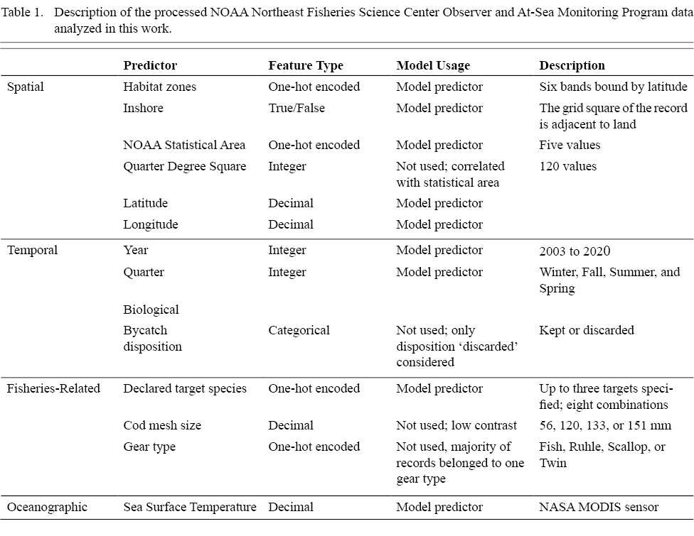
Table 1
We performed data processing on variables, which we term “features” following ML terminology, and observations (records) of the OSMP data (Fig. 2). Our initial quality control effort was made to remove unidentified, ambiguous (e.g., seaweed), and inanimate (e.g., wood and rocks) bycatch records. We then removed observations from 1994 to 2002, due to suspected inconsistent data collection protocols for those years, following our initial data evaluation. We also removed candidate features “gear type” and “cod mesh size”. We found that the representation of these features in the data was predominately composed of a single gear type and cod mesh size (Table 1). Records with impossibly large weights and those with latitude and longitude values outside of our spatial domain (e.g., those located on land) were also removed. We only used records of taxa that were discarded and observed. Finally, we extracted uninformative data columns, including row identifiers, columns with little contrast, and features with significant correlations to other features. We used linear and rank correlations to identify features that exhibited correlations of 0.90 or greater, keeping only one of the features in the model.
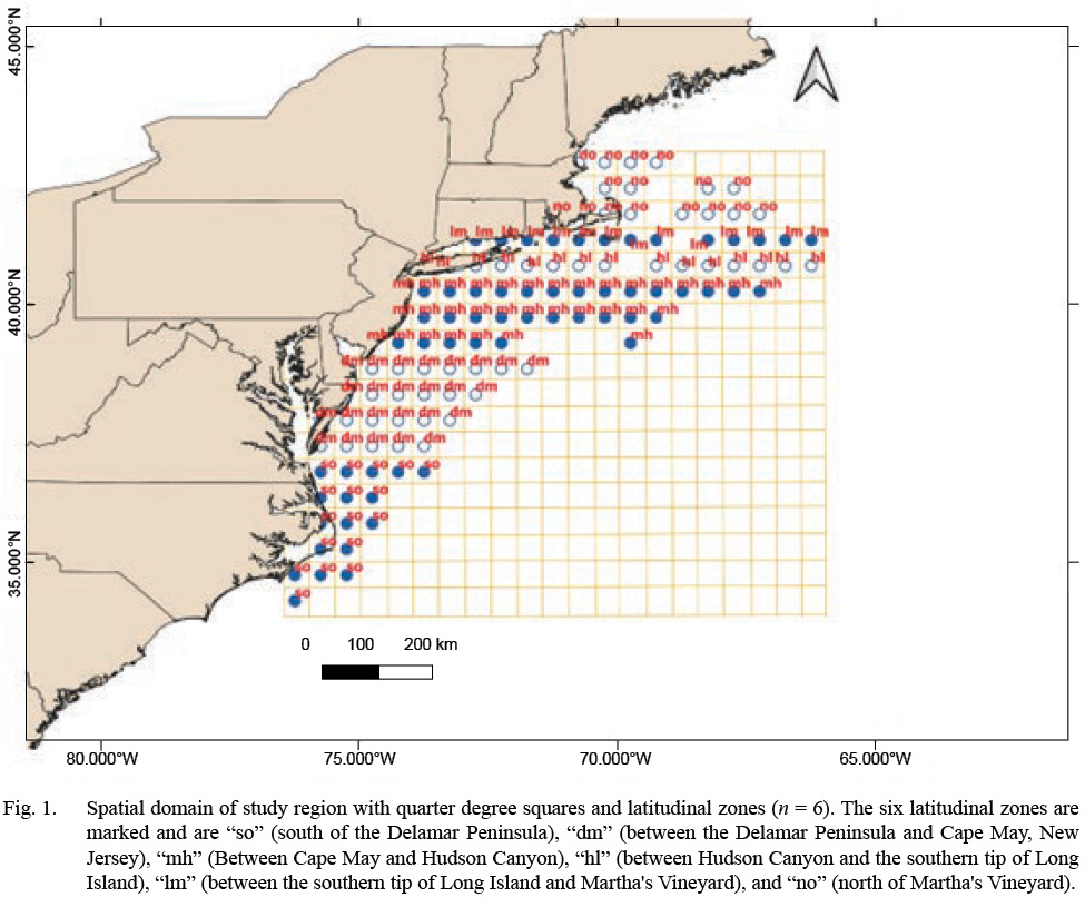
Fig. 1
Following the selection of informative features, we performed feature engineering to produce additional predictors (Table 1). All categorical features were one-hot encoded for conversion into numerical features to enable model runs (Yang et al., 2019). We defined six zones corresponding to regions of interest to commercial fishers in the region. Each zone comprised all OSMP records from grid squares bounded by latitudinal bands within the spatial domain of the study area. Latitudinal zones were“South of the Delamar Peninsula,”“Between the Delamar Peninsula and Cape May,”“Between Cape May and Hudson Canyon,”“Between Hudson Canyon and the southern tip of Long Island,”“Between the southern tip of Long Island and Martha's Vineyard,” and “North of Martha's Vineyard” (Fig. 1). We engineered a categorical feature such that the quarter-degree grid squares were designated as inshore if the square intersected with any land and offshore otherwise. We developed quarterly estimates of sea surface temperature (SST) at the spatial resolution (0.25° × 0.25° grid squares) of the OSMP data. Sea surface temperature estimates were obtained from the ocean-color images available from Moderate Resolution Imaging Spectroradiometer (MODIS) sensor (https://modis.gsfc.nasa.gov/data/). Data from this sensor provided an uninterrupted time series of ocean color images for the duration of the OSMP data. We used level-3 processed data at 9 km and monthly spatial and temporal resolutions. These data were used to develop monthly grid-square (0.25° × 0.25° grid squares) values of mean SST. Finally, we engineered a feature to represent the trip's declared target(s). The record included primary, secondary, and tertiary target species in other trips. The reported target for the trip was the combination of the stated target species. In some cases, only a single species was the declared target.
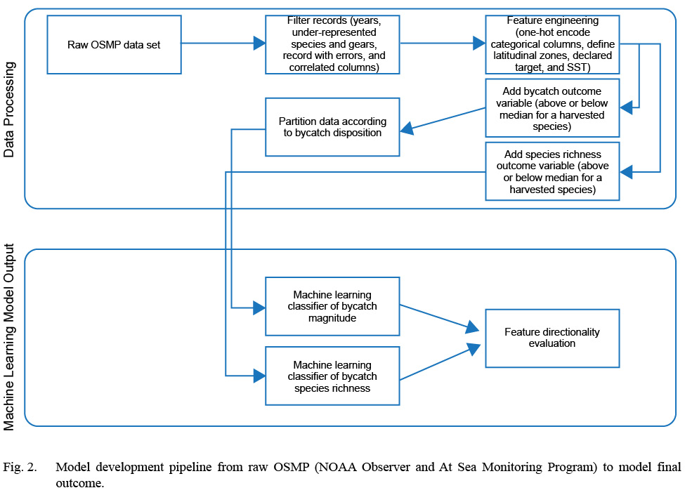
Fig. 2
We developed two features as the responses for analysis. The first was a binary categorical feature that indicated if the weight of the bycatch taxa for that trip was greater than or less than the median of the weight of that bycaught taxa for all trips. We removed taxa found in a percentage of records less than 0.5% to develop this feature. We then log-transformed the weight of each record. The taxonomic group-specific median of the log-transformed weight was determined to produce the binary categorical feature. A one was assigned if the value of the group was greater or equal to the value of the taxa-specific median, and a zero otherwise. The full data set was then partitioned by the declared primary target of the fishing trip: Summer Flounder, Scup, Black Seabass, or Longfin Squid (Table 2). The partitioning resulted in four groups of data for analysis of bycatch weight. The second analysis was a binary categorical feature that indicated if the richness (number of taxa) of bycatch for that trip was greater than or less than the median of the richness for all trips. The taxonomic group-specific median number of species was determined, and a one was assigned if the value of the group was greater or equal to the value of the taxa-specific median value and a zero otherwise.
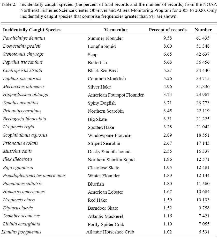
Table 2
We used a gradient-boosting ensemble machine learning algorithm to classify the categorical outcome features for bycatch weight and taxonomic richness. Gradient boosting was used because it captures complex non-linear dependencies at a low computational cost, especially for data with a low signal-to-noise ratio (Friedman, 2001). Gradient boosting was also used for transparency and ease of the interpretability of results (Arrieta et al.,< 2020). For model training, a random subset of 70% of data records was used as a training set, and the remainder was used for model testing. The best number of boosting trees and their depths were determined using cross-validation. The Adaboost loss function was used for the model optimizer, decision tree stumps were the base learner, and subsampling was the regularization method. Model performance evaluation metrics were classification accuracy, recall, precision, and F1 scores (Natekin and Knoll, 2013). We evaluated accuracy using a confusion matrix and provided information to understand how the frequency of the predicted classification compares to the frequencies observed in the data. The recall is the ratio of the frequency of the true positive to the sum of the true positive’s frequency and the false negative’s frequency. Recall indicates the proportion of the actual positives the model correctly identified. Similarly, precision is the ratio of the frequency of the true positive to the sum of the true positive’s frequency and the false positive’s frequency. The precision measurement’s value indicates the model’s correctness level for those predicted to be positive. The F1 value is a function combining precision and recall:

The F1 score balances the precision and recall estimates, correcting for the uneven distribution of observed classes.
Because an ensemble of trees was used as the underlying algorithm for each model, result transparency can be a challenge (Du et al., 2019). Two techniques were used to interpret and understand the classification outcome as a function of spatial, temporal, and biological features. We first calculated the feature importance metric. Measures of feature importance allow an understanding of how much of the variability in a model is ascribed to a specific candidate feature. Only features contributing to predictions in at least 2% of cases were considered. We used gain to estimate feature importance metric. This estimates how effective each feature is at improving accuracy in the prediction. The second approach used in this study to understand classification outcomes was the shapley additive explanation method (termed SHAP). This metric is a theoretic approach to model explainability (Lundberg and Lee, 2017). We calculated SHAP values to understand the directionality of feature importance. A visualization for SHAP values was used as a qualitative tool to assess feature importance and associated data influence on model performance. The approach allowed visualiztion of whether an observation of a feature on model prediction was high or low (horizontal position on graph) and the magnitude of that same observation (a grayscale value for the observation point).
Results
The analysis of bycatch patterns in the Summer Flounder, Scup, Black Seabass, and Longfin Squid fisheries indicated that six species of living marine resources were incidentally caught in more than 5% of the records (see Table 2). These species were Summer Flounder, Longfin Squid, Scup, Butterfish (Peprilus triacanthus), Black Sea Bass, and Common Monkfish (Lophius piscatorius). An additional 25 species were found in at least 1% of the records. These were a diverse group of taxa, including cartilaginous fishes (e.g., Spiny Dogfish, Big Skate, Dusky Smooth-hound, and Clearnose Skate), crustaceans (American Lobster and Portly Spider Crab), chelicerate arthropods (Atlantic Horseshoe Crab), and bony fishes. Less than 1% of the taxa accounted for 22.0% of the total number of records, including crabs, rays, flounders, and scallops.
The most commonly occurring bycatch in terms of frequency of records was the same as the declared primary target of the trip each fishery. The exception was for the Longfin Squid fishery, in this fishery Butterfish, Spotted Hake, Windowpane Flounder, and Silver Hake were the primary bycatch. For all years evaluated, the fisheries targeting Summer Flounder had the largest discards (1 539.1 MT), followed by fisheries for Longfin Squid (1 189.7 MT), Scup (498.9 MT), and Black Sea Bass (312.0 MT; Table 3). For all four fisheries, discards followed a species-specific pattern. For the Summer Flounder, Sea Bass, and Scup fisheries, spiny dogfish (Squalus acanthias) comprised the majority of discards and were present in each. Spotted Hake (Urophycis regia) is a dominant bycatch species for the Longfin Squid fishery. The greatest number of incidentally caught taxa in greater than 5% of records were found in the Summer Flounder fishery, with seven, and the smallest in the Longfin Squid fishery, with four. The directed fisheries for the Black Seabass and Scup fisheries exhibited six taxa each in greater than 5% of the records. Species of non-commercial interest commonly occurred in each fishery examined included skates, sea robins, and flatfishes (Table 3).
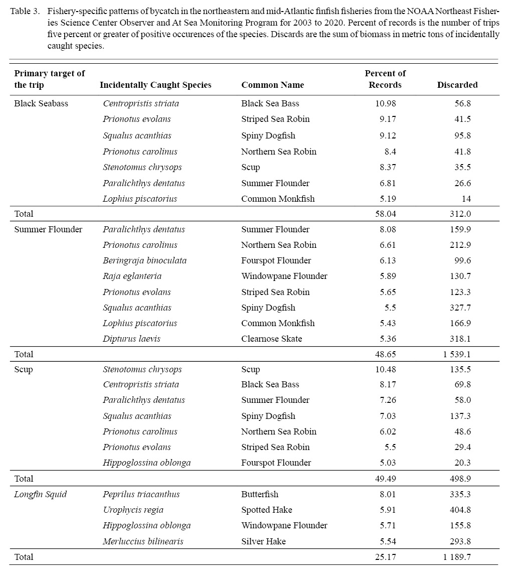
Table 3
Model accuracies were generally consistent for each fishery, and there were no discrepancies between accuracy and the other performance metrics. Model classification accuracy was greatest for the Summer Flounder fishery (0.73), and recall was largest for the Longfin Squid fishery (0.75) for the above median classification of bycatch weight. The model performance metrics were consistently greater for taxonomic richness classification than for bycatch weight classification in each of the four fisheries (Table). The number of model features was greatest for Longfin Squid (n = 269), followed by Summer Flounder (n = 263) for the bycatch classification model. The data set for the classification model of taxonomic richness had the fewest number of records (10 084) and the fewest number of features (n = 82).
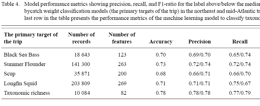
Table 4
Different spatial, temporal, biological, and fishery features were identified as important in classifying the magnitude of taxa-specific bycatch in the four fisheries examined. Across all models, the oceanographic feature sea surface temperature and the temporal feature year were the most important factors in classifying the median weight of bycatch (Figs. 3 to 6). Among the spatial features, longitude was ranked among the top four important features in all models, while latitude was present but ranked lower in importance. The spatial features “inshore” and “Area Southern Massachusetts” were only significant in predicting the median weight of bycatch for the Longfin Squid fishery model (Fig. 6). The biological features important in classifying bycatch magnitude in the Summer Flounder fishery included the presence or absence of cartilaginous fishes such as Clearnose Skate, Barndoor Skate, and Winter Skate as well as Spiny Dogfish (Fig. 3 to 6). The presence or absence of Spiny Dogfish was also important in classifying bycatch in the Black Seabass and Scup models (Figs. 4 and 5). In the Black Seabass classification model, three fishery features reflecting the absence of a secondary declared target species (ranked sixth), a declared secondary target of Southern Flounder (ranked eighth), and a declared secondary target of Scup (ranked ninth) were found to be important (Fig. 4A).
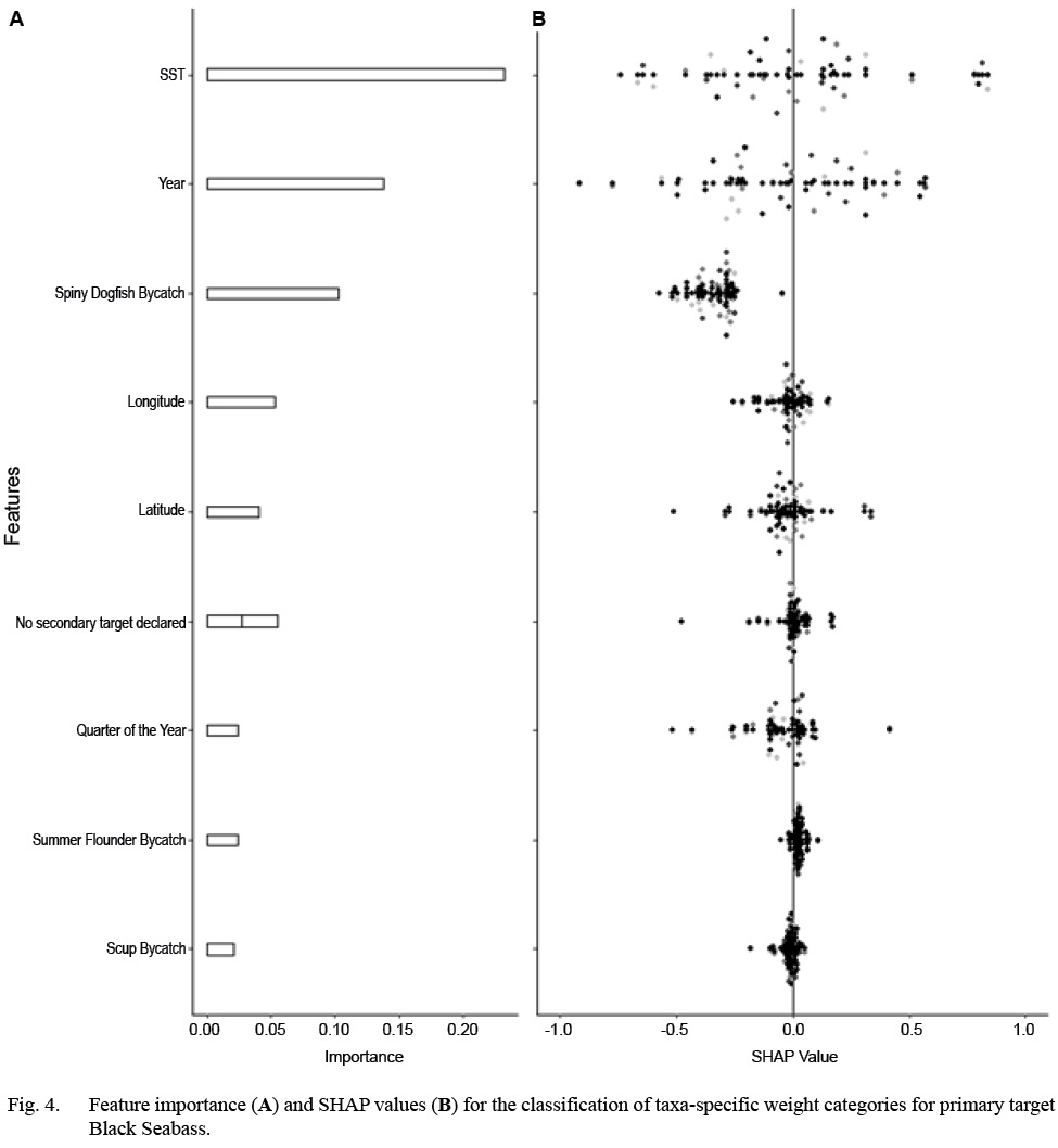
Fig. 4
The SHAP analysis was informative for some features but less informative for others. Although we observed that the feature sea surface temperature consistently ranked as the most important feature in all classification models, our SHAP analysis did not indicate a clear pattern in its direction of influence on the model outcome. High and low sea surface temperature values had positive and negative impacts on the predicted outcome. Conversely, the biological features representing specific bycatch species negatively influenced the model outcome, implying a tendency for the model to predict below median bycatch weight if these taxa were also present on the trip. We observed that only a few high observations exerted a highly positive influence. For each fishery’s bycatch classification model, the SHAP values for the temporal feature year indicated that more recent years positively impacted the model outcome (Figs. 3 to 6 and 8). For Black Seabass and Scup bycatch classification models, records with more recent years were classified as having greater than median bycatch. We found that the feature quarter of the year negatively influenced the predicted outcome, where greater than median bycatch weights were observed early in the year. Among the spatial features, the SHAP values for the feature longitude indicated a negative impact on the model outcome for feature values, with greater bycatch magnitudes occurring in the eastern parts of the geographic domain. For the feature longitude, SHAP values indicated that more easterly values tended to have positive impacts (greater than median bycatch weight) on the model outcome for Black Seabass and Scup. Scup and Longfin Squid’s feature longitude indicated that the geographic domain’s eastern regions had reduced bycatch. Features reflecting inshore fishing locations and fishing in Southern Massachusetts negatively impacted bycatch in the Longfin Squid classification model. Scup was the only model in which the presence of its species (Scup) was an important biological feature representing bycatch (Figs. 4 to 6).
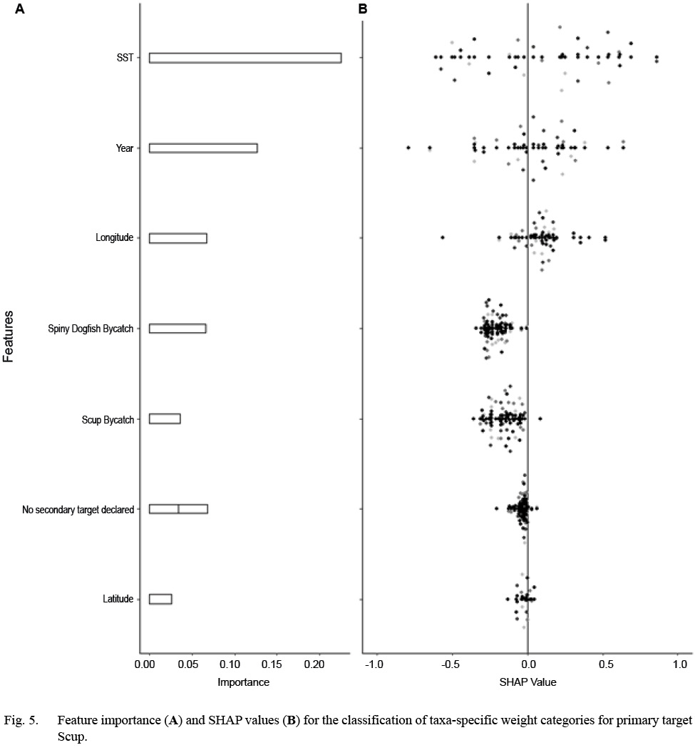
Fig. 5
The relationship between the number of records from a square grid location and taxonomic richness showed a positive, non-linear trend (Fig. 7A). The maximum taxonomic richness observed was 192 taxa, with a median of 75 and a minimum of 5 taxa. The highest richness was found in quarter-degree grid squares located offshore in the southern part of the study area, ranging from 37 to 41° N and -76 to 70° W (Fig. 7B). Conversely, the lowest richness was observed north and south of this region. For the model predicting taxonomic richness, sea surface temperature and year were consistently the most important features, indicating a trend of increasing richness in recent years (Fig. 8A). Longitude and latitude also played a role in the model, with richness increasing to the east and north (Fig. 8B). Additionally, the Longfin Squid bycatch feature had a positive influence on the model outcome, with increasing values of this feature leading to higher median richness.
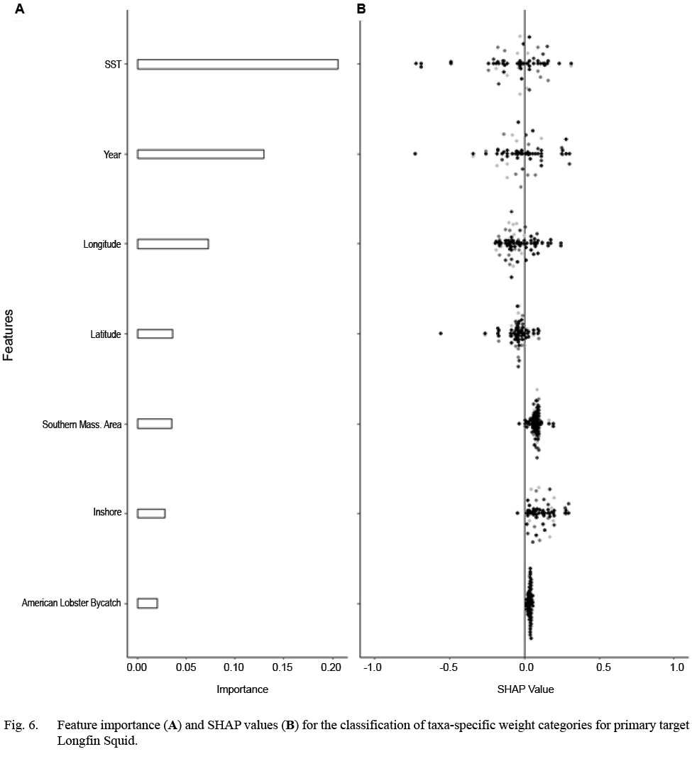
Fig. 6
Discussion
In this study, we examined the bycatch composition in four commercial fisheries in the northeastern U.S. We employed machine learning classification models to gain insights into the spatial, temporal, biological, and fishery characteristics that describe contrasts in fishery-specific bycatch magnitude and the richness of bycatch. Our primary findings indicate that six species each accounted for at least 5% of the records, including each targeted species. The observed bycatch magnitude for the four fisheries ranged from 312 to 1 539 mt over the 17-year data duration. We found that the binary classification accuracies of the models were only moderate, never exceeding 80% classification accuracy. All classification models consistently showed that the oceanographic feature sea surface temperature and the temporal feature year are important in determining model performance. Feature importance, however, does not provide an indication of the direction of the response. The SHAP analysis indicated little consistent pattern in the value of the response. The findings of this study show the promise and challenges of using ML approaches for describing contrasts in bycatch abundance and taxonomic richness for mobile gear fisheries in the mid-Atlantic. The benefits of using an ML approach in this case is that we do not need to rely ona priori models to describe the phenomena to be studied. ML approaches are “model agnostic”.
The contrast in the features that detect the importance of bycatch magnitude reflects differences in the nature of each of the fish stocks. The feature importance analysis for the Scup model indicated that the presence of Scup was an important biological feature that predicts bycatch. This finding implies that Scup catch has a very large component of discarded Scup. This is a well-documented concern in the mid-Atlantic and has necessitated management intervention. Indeed, gear restrictions and time-area closures have been implemented in the mid-Atlantic to reduce discarding Scup below the minimum legal size limit (Powell et al., 2004). In addition, for the classification of bycatch in the Scup fishery, the SHAP values of the category shark (a multi-taxa feature that includes all elasmobranchs) showed a positive impact, and Longfin Squid, a negative association with the above-median bycatch weight class. A co-occurrence of sharks and Scup, together with distinct habitat segregation with Longfin Squid, might be expected for Scup. The classification model of discard bycatch for the Black Seabass fishery was positively associated with the shark and sea robin species categories and negatively with the Longfin Squid category. Records of Black Seabass discard weight greater than the median were associated with bycatch of species from the shark, sea robin, and Longfin Squid categories, potentially reflecting Black Seabass co-occurrence with the latter two fish species. The co-occurrence of Black Sea Bass and sharks may be trophically related. The Northeast Fisheries Science Center (NEFSC) food habits database lists spiny dogfish (Squalus acanthias), Atlantic angel shark (Squatina dumeril), and a variety of skates as predators of Black Sea Bass (Steimle et al., 1999). Greater biomass of discarded Summer Flounder as bycatch was accompanied by lower catches of Longfin Squid, hakes, and Scup. A possible explanation for the negative association is interactions between gear selectivity and seasonal changes in species distribution leading to separation in the distribution of demersal fish (Shepherd and Terceiro, 1994; Gabriel, 1996; Link et al., 2002). Small-scale changes in habitat use within an area and season have been reported for Scup and Summer Flounder, where one species inhabits sandy bottoms and the other occupies complex hard bottom habitats (Shepherd and Terceiro, 1994). Such patterns of occurrence and habitat preferences may account for the observed associations in the Summer Flounder observations. In the analysis of bycatch in the Longfin Squid fishery, only the category Longfin Squid was negatively associated with the above-median bycatch class. Discards of Longfin Squid in that fishery indicate that the harvest of small or unmarketable Longfin Squid is responsible for this pattern. We note that of the fishery-related predictors, only the declared target species (or combination of species) if a secondary and or tertiary species were reported. Due to the constraints of the data available to the authors, it was not possible to analyze the impacts of cod mesh size and gear type.
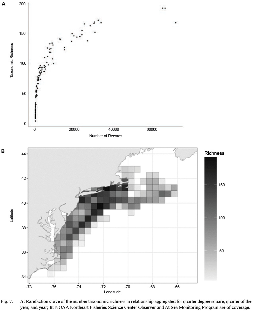
Fig. 7
We found some patterns in species richness observed from the bycatch analysis. Primarily, we saw an increase in richness from 2018 onwards. Alternatively, low species richness was associated with longitude toward the western areas and offshore habitats in the spatial domain of the study. This latter was expected, as offshore habitats may offer less habitat complexity and species richness than habitats closest to shore. Features reflecting spatial distribution were not always intuitive. For the species richness classification model, an increase in richness is predicted easterly, and north in the study domain was counter-intuitive. One explanation for this result might be that interactions between gear selectivity and seasonal changes in species distribution lead to the segregation of species-specific populations of demersal fish (Shepherd and Terceiro, 1994; Gabriel, 1996; Link et al., 2002).
SHAP values for each feature are presented to elucidate the relationship between feature magnitude and directionality on the outcome of regression tree models (Lundberg and Lee, 2017). Although important features in most models, sea surface temperature and year were suggestive of uncertain influence on directionality. This was an unexpected result. The feature engineering that we performed, to include sea surface temperature was done because we hypothesized that contrasts in bycatch magnitude could be described by this feature. That the SHAP analsyis indicated no consistency in the direction of this feature means that the feature was represented many times in the classification tree but that the predicted effect was contingent not on high and low values of sea surface temperatures. Instead, small increments in sea surface temperature lead to predictions of higher and lower than the median of bycatch weight. Similarly, the feature year may be considered a proxy for various interactive biological and abiotic processes. Like sea surface temperature, individual year values lead to processes that both increase or decrease taxa-specific bycatch magnitude. Conversely, although not as important for classification, biological features did indicate some direction of response. For example, features reflecting bycatch species were largely positive in their directionality, implying an expectation of a positive relationship between the targeted species’ weight and the weight of associated bycatch. The challenge is to make these associations actionable in a management context. Evaluation of bycatch composition of observer data in a multivariate framework could lead to insights into patterns of community composition of bycatch. That the spatial features “inshore” and “Area Southern Massachusetts” were a significant feature in predicting the median weight of bycatch for the Longfin Squid fishery model is more actionable.
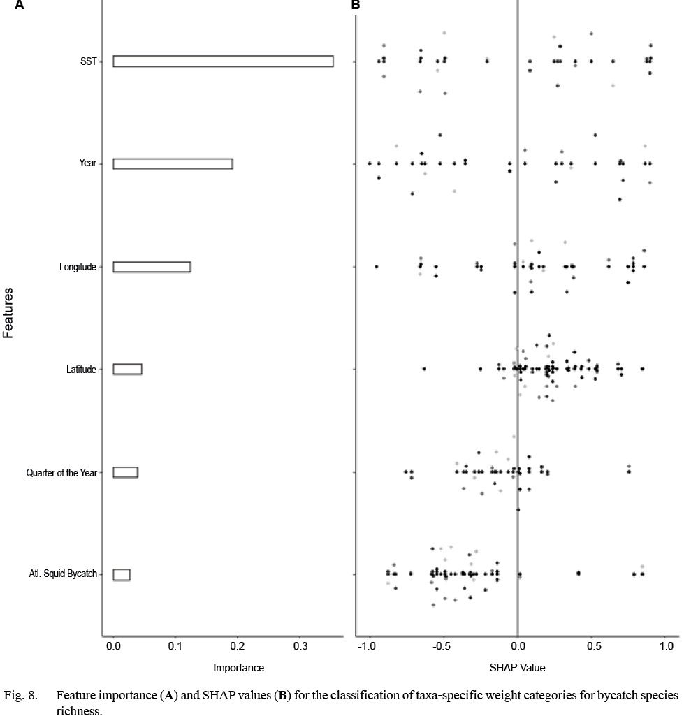
Fig. 8
The findings of this study point to the promise of using ML approaches for describing contrasts in bycatch data for fisheries in the mid-Atlantic using abundance and taxonomic richness metrics. The results of this study indicate that ML alternatives may successfully supplement traditional analytical approaches to fisheries research. Results from ML model runs captured generally expected patterns in the harvest according to target species. Given the inherent uncertainty associated with fisheries data, these results encourage adopting ML techniques to the field. However, adopting ML into the fisheries field must be done carefully, always with the analytical objective in mind. Adopting ML techniques blindly, without consideration of method explainability, may be a fruitful approach if classification is the only goal. ML techniques are best used in conjunction with traditional statistical analyses. These hypothesis-driven approaches allow model explanations.
Even with the encouraging results from the gradient-boosting ML approach used in this study, suggestions for further improvements may be offered. Fine-grained vessel positioning may aid fisheries management decisions by better classifying movement patterns into activities associated with fishing and non-fishing practices. A limitation of this study rests on the high level of data aggregation provided by the onboard observation program. With less aggregation, data at trip levels, for example, more fine-grained, robust results would be possible, and better estimates of the effects of biological features could have been provided. Another limitation of complex resolution is observer coverage. Due to the high costs associated with observer programs, the spatial and temporal range may be insufficient to detect fine-grained results necessary for optimal fisheries management. Model quality of machine learning is contingent on data availability.
Additional benefits from this study may be achieved from an undertaking aimed at the automation of bycatch estimates, especially concerning the limitations above of observer coverage. With the advent of affordable, off-the-shelf global positioning devices, detailed information on the spatial dynamics of fishing efforts may be accurately estimated with classifiers as used in this study for small- and large-scale fisheries worldwide. Moreover, equipping vessels with cameras may also assist in assessing bycatch amounts. Camera images may be readily analyzed with computer vision approaches, such as deep learning algorithms (LeCun et al., 2015), to automate data collection, allowing for widespread coverage of bycatch data (Khokher et al., 2021). Computer vision has been successfully used in fish identification (Ditria et al., 2020), estimation of fish abundance (Tseng and Kuo, 2020), and length distributions (White et al., 2006), often surpassing the accuracy of human experts.
Machine learning approaches to analyzing fisheries data will likely not replace traditional modeling methods. In combination, formal modeling and ML may capture enough of the complexities and dynamics of ecological processes determining catch abundances to provide robust advice for sustainable harvest. A trend in augmenting the performance of traditional fisheries stock assessment and estimation models using ML has been observed recently (Pérez-Ortiz et al., 2013; Syed and Weber, 2018; Kaemingk et al., 2020; Yang et al., 2020; Chan and Pan, 2021), attesting to the applicability of ML algorithms to fisheries data. With the increasing prospect of automation in fisheries data collection, ML techniques may be the only feasible approach for data processing and analysis as datasets become more complex. Automation, however, comes with the cost of transparency, primarily when deep learning techniques are used for classification. Because decisions based on such analysis most likely will have significant ecological, economic, and social impacts, explaining the results of ML techniques clearly and understandably is a must. Many ML techniques are defined as opaque, whereby how results are obtained is not clearly understood. Using mechanisms for explaining the results of an analysis, as done in this study, must accompany any opaque ML technique if the benefits of this new and ever-growing analytical alternative are to be fully realized.
References
Alverson D. L., Freeberg M. H., Murawski, S. A., Pope, J. G. 1994. A Global Assessment of Fisheries Bycatch and Discards. Food and Agriculture Organization of the United Nations.
Arrieta, A., Díaz-Rodríguez, N., Del Ser J., Bennetot, A., Tabik S., Barbado, A., Garcia, S., Gil-Lopez, S., Molina, D., Benjamins, R., Chatila, R., and Herrera, F. 2020. Explainable Artificial Intelligence (XAI): Concepts, taxonomies, opportunities and challenges toward responsible A.I. Inf. Fusion, 58: 82–115. https://doi.org/10.1016/j.inffus.2019.12.012
Batsleer, J., Hamon, K. G., van Overzee, H. M. J., Rijnsdorp, A. D., and Poos, J. J. 2015. High-grading and over-quota discarding in mixed fisheries. Reviews in Fish Biology and Fisheries, 25: 715–736. https://doi.org/10.1007/s11160-015-9403-0
Baum, J. K., and Worm, B. 2009. Cascading top-down effects of changing oceanic predator abundances. J Anim Ecol. 78: 699–714. https://doi.org/10.1111/j.1365-2656.2009.01531.x
Bellido, J. M., Santos M. B., Pennino, M.G., Valeiras, X., and Pierce G.J. 2011. Fishery discards and bycatch: solutions for an ecosystem approach to fisheries management? Hydrobiologia, 670: 317–333. https://doi.org/10.1007/s10750-011-0721-5
Chan, H. L., and Pan, M. (2021) Fishing trip cost modeling using generalized linear model and machine learning methods – A case study with longline fisheries in the Pacific and an application in Regulatory Impact Analysis. PLOS ONE 16:e0257027. https://doi.org/10.1371/journal.pone.0257027
Davies, R. W. D., Cripps, S. J., Nickson, A., and Porter, G. 2009.Defining and estimating global marine fisheries bycatch. Mar Policy, 33: 661–672. https://doi.org/10.1016/j.marpol.2009.01.003
Ditria, E. M., Lopez-Marcano, S., Sievers, M., Jinks, E. L., Brown, C.J., and Connolly, R. M. 2020. Automating the Analysis of Fish Abundance Using Object Detection: Optimizing Animal Ecology With Deep Learning. Front Mar Sci,. 7: https://doi.org/10.3389/fmars.2020.00429
Du, M., Liu, N., and Hu, X. 2019. Techniques for interpretable machine learning. Commun ACM, 63: 68–77. https://doi.org/10.1145/3359786
Dunn, D. C., Boustany, A. M., Roberts, J. J., Brazer, E., Sanderson, M., Gardner, B., and Halpin, P. N. 2014. Empirical move-on rules to inform fishing strategies: A New England case study. Fish and Fisheries, 15: 359–375. https://doi.org/10.1111/faf.12019
Friedman, J. H. 2001. Greedy function approximation: A gradient boosting machine. Ann. Stat., 29: 1189–1232. https://doi.org/10.1214/aos/1013203450. https://doi.org/10.1214/aos/1013203451
Gabriel, L. 1996. The Role of Targeted Species in Identification of Technological Interactions in Mid-Atlantic Bight Groundfish Fisheries. J. Northwest Atl. Fish. Sci., 19: 11–20. https://doi.org/10.2960/J.v19.a1
Gilman, E., Perez Roda, A., Huntington,T., Kennelly, S. J., Suuronen, P., Chaloupka, M., and Medley, P. A. H. 2020.Benchmarking global fisheries discards. Sci. Rep. 10: 14017. https://doi.org/10.1038/s41598-020-71021-x
Heath, M. R, Cook, R. M, Cameron, A. I., Morris, D. J., and Speirs, D. C. 2014. Cascading ecological effects of eliminating fishery discards. Nat. Commun., 5: 3893. https://doi.org/10.1038/ncomms4893
Jordan M. I. , and Mitchell, T. M. 2015. Machine learning: Trends, perspectives, and prospects. Science, 349: 255–260. https://doi.org/10.1126/science.aaa8415
Kaemingk, M. A., Hurley, K. L., Chizinski, C. J., and Pope, K. L. 2020. Harvest–release decisions in recreational fisheries. Can. J. Fish. Aquat. Sci., 77: 194–201. https://doi.org/10.1139/cjfas-2019-0119
Kelleher, K. 2005. Discards in the World’s Marine Fisheries: An Update. Food and Agriculture Organization of the United Nations. Rome. 131 p.
Khokher, M. R., Little, L. R., Tuck, G. N., Smith, D. V., Qiao, M., Devine, C., O’Neill, H., Pogonoski, J.J., Arangio, R., and Wang, D. 2021. Early lessons in deploying cameras and artificial intelligence technology for fisheries catch monitoring: where machine learning meets commercial fishing. Can. J. Fish. Aquat. Sci., 79: 1–10. https://doi.org/10.1139/cjfas-2020-0446
LeCun, Y., Bengio, Y., and Hinton, G. 2015. Deep learning. Nature, 521: 436–444. https://doi.org/10.1038/nature14539
Leipzig, J., Bakis, Y., Wang, X., Elhamod, M, Diamond, K., Dahdul, W., Karpatne, A., Maga, M, Mabee, P., Bart H. L., and Greenberg, J. 2021. Biodiversity Image Quality Metadata Augments Convolutional Neural Network Classification of Fish Species. bioRxiv 2021.01.28.428644. https://doi.org/10.1101/2021.01.28.428644
Link, J. S., Bundy, A, Overholtz, W. J., Shackell, N., Manderson, J., Duplisea, D., Hare, J., Koen-Alonso, M., and Friedland K. D. 2011. Ecosystem-based fisheries management in the Northwest Atlantic. Fish. and Fish. 12: 152–170. https://doi.org/10.1111/j.1467-2979.2011.00411.x
Link, J. S, Garrison, L. P., and Almeida, F. P. 2002. Ecological Interactions between Elasmobranchs and Groundfish Species on the Northeastern U.S. Continental Shelf. I. Evaluating Predation. North. Am. J. Fish. Manag. 22: 550–562. https://doi.org/10.1577/1548-8675(2002)022%3C0550:EIBEAG%3E2.0.CO;2
Lundberg, S. M., and Lee, S.-I. 2017. A Unified Approach to Interpreting Model Predictions. NIPS'17: Proceedings of the 31st International Conference on Neural Information Processing Systems. 4768–4777.
Natekin, A., and Knoll, A. 2013. Gradient boosting machines, a tutorial. Front Neurorobotics, 7: 21. https://doi.org/10.3389/fnbot.2013.00021
Northeast Fisheries Science Center (2010) Fisheries observer program manual. 442p.
O’Keefe, C. E., Cadrin, S. X., and Stokesbury, K. D. E. 2014.Evaluating effectiveness of time/area closures, quotas/caps, and fleet communications to reduce fisheries bycatch. ICES J. Mar. Sci. 71: 1286–1297. https://doi.org/10.1093/icesjms/fst063
Pérez-Ortiz, M., Colmenarejo, R., Fernández Caballero, J. C., and Hervás-Martínez, C. 2013. Can Machine Learning Techniques Help to Improve the Common Fisheries Policy? 278–286. https://doi.org/10.1007/978-3-642-38682-4_31
Pikitch, E., Sandtora, C., Babcock, E., Bakun, A., Bonfil, A., Conover, D., Dayton, P., Doukakis, P., Fluharty, D., Heneman, B., Houde, E., Link, J, Livingston, P., Mangel, M., McAllister, M., Pope, J., and Sainsbury, K. 2004.Ecosystem-Based Fishery Management. Science, 305: 346–347. https://doi.org/10.1126/science.1098222
Poos, J. J., Bogaards, J. A., Quirijns, F. J., Gillis, D. M., and Rijnsdorp, A. D. 2010. Individual quotas, fishing effort allocation, and over-quota discarding in mixed fisheries. ICES Journal of Marine Science, 67: 323–333. https://doi.org/10.1093/icesjms/fsp241
Powell, E. N., Bonner, A. J., Muller, B., and Bochenek, E. A. 2004. Assessment of the effectiveness of scup bycatch-reduction regulations in the Loligo squid fishery. Journal of Environmental Management, 71: 155–167. https://doi.org/10.1016/j.jenvman.2003.12.016
Savoca, M. S., Brodie, S., Welch, H., Hoover, A., Benaka, L. R., Bograd, S. J., and Hazen, E. L. 2020. Comprehensive bycatch assessment in U.S. fisheries for prioritizing management. Nat. Sustain. 3: 472–480. https://doi.org/10.1038/s41893-020-0506-9
Scheffer, M., Carpenter, S., and de Young, B. 2005. Cascading effects of overfishing marine systems. Trends Ecol. Evol. 20: 579–581. https://doi.org/10.1016/j.tree.2005.08.018
Shepherd, G. R., and Terceiro, M. 1994. The Summer Flounder, Scup, and Black Sea Bass Fishery of the Middle Atlantic Bight and Southern New England Waters. http://aquaticcommons.org/id/eprint/2693
Steimle, F. W., Morse, W. W., and Johnson, D. L. 1999. Goosefish, Lophius americanus, life history and habitat characteristics. Essential Fish Habitat Source Document, NMFS-NE-127. Northeast Fisheries Science Center, Highlands, NJ.
Suuronen, P., and Gilman, E. 2020. Monitoring and managing fisheries discards: New technologies and approaches. Mar. Policy, 116: 103554. https://doi.org/10.1016/j.marpol.2019.103554
Syed, S., and Weber, C. T. 2018. Using Machine Learning to Uncover Latent Research Topics in Fishery Models. Rev. Fish. Sci. Aquac., 26: 319–336. https://doi.org/10.1080/23308249.2017.1416331
Tseng, C.-H., and Kuo,. Y-F. 2020. Detecting and counting harvested fish and identifying fish types in electronic monitoring system videos using deep convolutional neural networks. ICES J. Mar. Sci. 77: 1367–1378. https://doi.org/10.1093/icesjms/fsaa076
Viana, D., de Souza M. R. D. P.., de Assis Teixeira da Silva, U., Pereira, D. M. C., Kandalski, P. K., Neundorf, A. K. A., Peres, D., dos Santos, A. T., Romão, S., Moura, M. O., Fávaro, L. F., and Donatti, L. 2021. The effect of bottom trawling time on mortality, physical damage and oxidative stress in two Sciaenidae species. Rev. Fish. Biol. Fish. 31: 957–975. https://doi.org/10.1007/s11160-021-09682-8
White, D. J., Svellingen, C., and Strachan, N. J. C. 2006.Automated measurement of species and length of fish by computer vision. Fish. Res. 80: 203–210. https://doi.org/10.1016/j.fishres.2006.04.009
Yang, K. K., Wu, Z., and Arnold, F. H. 2019. Machine-learning-guided directed evolution for protein engineering. Nat. Methods, 16: 687–694. https://doi.org/10.1038/s41592-019-0496-6
Yang, S., Dai ,Y., Fan, W., and Shi, H. 2020 . Standardizing catch per unit effort by machine learning techniques in longline fisheries: a case study of bigeye tuna in the Atlantic Ocean. Ocean Coast. Res. 68: https://doi.org/10.1590/s2675-28242020068226
Citation: Riedel, R. and Leaf, R. 2023. Analysis of bycatch patterns in the northeastern USA finfish trawl fisheries. J. Northw. Atl. Fish. Sci., 54: 31–48. https://doi.org/10.2960/J.v54.m741