J. Northw. Atl. Fish. Sci., Vol. 50: 37–50
Michael P. Torre, Kisei R. Tanaka, and Yong Chen
University of Maine, School of Marine Sciences,Orono, Maine, 04469, USA
Michael.Torre@Maine.edu
Corresponding Author: Michael P. Torre
Torre, M.P., K.R. Tanaka, and Y. Chen. 2019. Development of a climate-niche model to evaluate spatiotemporal trends in Placopecten magellanicus distribution in the Gulf of Maine, USA. J. Northw. Atl. Fish. Sci., 50: 37–50. https://doi.org/10.2960/J.v50.m721
Abstract
We developed a climate-niche species distribution model to evaluate spatiotemporal trends in Atlantic sea scallop (Placopecten magellanicus) along the coastal waters of the Gulf of Maine. We used a Tweedie-generalized additive model (GAM) to quantify the relationships between scallop abundance and key environmental variables. A boosted regression tree was used to identify significant interactions among environmental variables to integrate within the Tweedie GAM and a regional circulation model was incorporated with the Tweedie GAM to hindcast projections of scallop distribution and assess the impacts of environmental change on this species. Additionally, we evaluate two common model fitting and variable selection methods for GAMs to ensure high model performance. A classic backward variable selection procedure was compared to penalized thin plate regression splines. Projections from the climate-niche species distribution model show higher scallop density along inshore areas relative to those farther offshore. An increasing temporal trend in scallop density was observed along inshore areas and a decreasing temporal trend was observed in areas farther offshore. Additionally, we found that the GAM incorporating thin plate regression splines outperformed the widely used backwards stepwise procedure. This modeling framework will help to inform adaptive management strategies for the scallop fishery within the context of a changing Gulf of Maine ecosystem.
Keywords: Species distribution models, generalized additive models, model selection, Placopecten magellanicus, Gulf of Maine
PDF
Download Citation Data

Citation to clipboard
 Reference management software (Endnote, Mendeley, RefWords, Zotero & most other reference management software)
LaTex, BibDesk & other specific software
Introduction
Atlantic sea scallops (Placopecten Magellanicus) support a highly valuable fishery in the United States. However, the scallop fishery within Maine state waters is relatively depleted. The fishery there bottomed out in 2005 when only 33 000 lb was taken, about 1% of what was landed in the early 1990s (Kelly 2012). However, recent years have shown an increasing trend in scallop abundance, with over 800 000 lb landed in 2018, allowing for an opportunity to establish a persistent, valuable fishery through research-informed management and conservation efforts (Kelly, 2012).
The distribution and abundance of species are central concepts to ecological research and vital components of conservation planning and fisheries management (Franklin, 2010). Species distributions are influenced by many interacting biotic and abiotic processes that can manifest as complex occurrence-environment relationships (Boulangeat et al., 2012; Merow et al., 2014). Thus, a key step in understanding the biogeography of species is identifying environmental factors that regulate the distribution of a species (Merow et al., 2014). Like most benthic species, scallop abundance and distribution are influenced by an array of interacting variables such as depth, current, temperature, and salinity (Stokesbury and Himmelman 1995, Hart and Chute 2004).
Throughout their geographic range, scallops occur mainly at depths of 15 to 110 m, but can be found as shallow as 2 m in the northern part of its range (Naidu and Anderson 1984, Carsen et al., 1995). Temperature is an important environmental factor influencing growth rates of this species with adult scallops showing optimal growth at temperature between 10–15°C and temperatures above 21°C being lethal (Stewart and Arnold 1994). This species prefers full strength seawater (~35 ppt), with salinities of 16.5 ppt or lower being lethal (Stewart and Arnold, 1994). Scallops are usually found in environments with strong currents (Hart and Chute, 2004), and flow velocity has been shown to be a key factor controlling waste removal, oxygen uptake, feeding, and growth rates (Stewart and Arnold, 1994; Shumway and Parsons, 2006). Optimal growth for this species occurs near 0.1 m s-1 (Wildish and Saulnier, 1992) and feeding inhibition has been observed to start at ~0.25 m s-1 (Pilditch and Grant, 1999). While the influence of key environmental variables on bivalve ecology is apparent, quantitative evaluations of scallop-environment relationships and spatiotemporal trends of distribution are uncommon (Shumway and Parsons, 2006; Mendo et al., 2014).
Water temperatures within the Gulf of Maine (GoM) have increased over the past 35 years at an average rate of 0.026°C yr -1 (Mills et al., 2013; Pershing et al., 2015). Rapidly increasing temperatures are changing the distribution of numerous marine species (Overholtz et al., 2011, Howell and Auster, 2012, Hollowed et al., 2013), with many fish stocks undergoing a poleward shift in their center of biomass and/or an increase in depth (Nye et al., 2009). Scallop distribution has also been shown to be impacted by climatic variability (Frank et al., 1990, Kurihara 2008). Dickie (1955) and Caddy (1979) demonstrated that higher temperatures in the Bay of Fundy were correlated with changes in scallop abundance. Additionally, climactic changes may alter larval development as well as the survival of juvenile and adult scallops (Dickie, 1955; Caddy, 1979). Considering a changing GoM ecosystem (Mills et al., 2013; Pershing et al., 2015), it is important to document the importance and potential synergistic effects of climate forcing on the dynamics of species abundance and distribution.
In this study, we use data describing the distribution of scallops in the GoM to develop a climate-niche species distribution model (SDM). This SDM predicts the spatial distribution of scallops within the inshore Gulf of Maine across unsampled areas and hindcasts spatiotemporal changes in the distribution of scallops from 2005–2013 to evaluate the effects of shifting environmental conditions on this species. We used Tweedie-generalized additive models (GAMs) to quantify the relationships between scallop abundance and key environmental variables. Additionally, we evaluate two prevalent model fitting and variable selection methods for GAMs to ensure high model performance. A classic backward variable selection procedure was compared to penalized thin plate regression splines following Wood (2003, 2006). This modeling framework will help to inform adaptive management strategies for the scallop fishery within the context of a changing GoM ecosystem.
Materials and Methods
Study Area and survey data.
Dredge-based fishery-independent scallop surveys conducted over 15 years, from 2005 to 2017, by the Maine Department of Marine Resources were used for this modeling effort (DMR: Kelly, 2012; Fig. 1). Survey coverage extends out to 3 nm from shore from southern Maine to the Maine-Canadian border, USA (Fig. 1). This dataset comprised two annual random systematic surveys, one in the spring survey covering alternating portions of inshore Maine waters and one in the fall covering select coastal areas. The gear used for both surveys is an unlined, 7 ft. New Bedford style drag with 2 in rings, 1.75 in head bale, 3.5 in twine top, 10 in pressure plate and rock chains. Since scallops <65 mm in shell height were not efficiently sampled with the 2 in rings (Kelly 2012), these were excluded from all analyses. Tows were conducted at 3.5–4 knots and lasted ~ 2.5 minutes. A total of 4 321 tows were made yielding 507 911 total observed scallops in this dataset (Fig. 2). All tows from the survey were included within the modeling framework. Scallop abundance from each tow was standardized to catch-per-unit-effort (CPUE) over a 2.5-minute tow.

Fig. 1
The GoM is characterized by a mixture of oceanic influences directly affected by the Labrador Current, the Gulf Stream, and the freshwater discharge from the St. Lawrence River (Tremblay 1997; Drinkwater and Gilbert, 2004). As such, water temperature follows a gradient moving up the coast and offshore. Within the study area, scallops were found where maximum yearly temperature ranged from 8°C in deeper areas to 16°C in shallow areas. Salinity ranged from 26 ppt in areas subject to freshwater inputs to full seawater (35 ppt) in offshore locations. The Maine covered depths to ~110 m, since scallops are uncommonly found outside of this depth range (Hart and Chute, 2004), with the majority of tows occurring in <60 m.
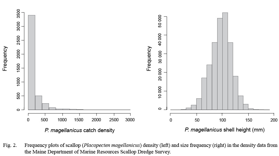
Fig. 2
Environmental data
Because the DMR surveys did not measure temperature, salinity, or current velocity, the Finite-Volume Community Ocean Model (FVCOM), a regional ocean circulation model developed by the University of Massachusetts-Dartmouth and the Woods Hole Oceanographic Institution (Chen et al., 2006) was used to simulate monthly estimates of bottom temperature, salinity, and current velocity from 2005 to 2013. It has a horizontal resolution ranging from 0.02 km to 10 km and captures complex and irregular coastal geometry, making it suitable for physical and biological studies in coastal regions and estuaries (Chen et al., 2011). FVCOM predictions were matched to survey tows from the nearest neighboring FVCOM node during time of sampling (Fig. 3). Horizontal current velocity was calculated to approximate the magnitude of water flow at a given FVCOM node. Current velocity C was estimated at station i, and year y from FVCOM predictions using the following equation:
 (1)
(1)
where C is the magnitude of the predicted current velocity and u and y are the x and y vector components of the velocity(Chen et al., 2011; Torre et al., 2018). Bathymetry data were obtained from the U.S. Coastal Relief Model (CRM) (National Geophysical Data Center, 1999).

Fig. 3
Generalized additive models
A generalized additive model (GAM) was used to make spatiotemporal predictions of scallop distribution in the inshore GoM (Fig. 3). Conceptually, GAMs are generalized linear models with a linear predictor upon which smooth functions are applied to covariates (Guisan et al., 2002, Marra and Wood, 2011). The strength of GAMs lie in their ability to handle, in a multivariate regression setting, non-linear and non-monotonic relationships between the response and covariates that arise often in nature (Guisan et al., 2002). Resulting from their ability to deal with a variety of distributions that occur in ecological data, the use of GAMs has been extensively applied to species distribution modeling efforts (Guisan et al., 2002, Sagarese et al., 2014, Young and Carr, 2015).
Terms included within the full model were selected according to boosted regression tree (BRT) analysis (Elith et al., 2008), and bivariate interaction terms were also identified and included based on this analysis. BRT models were used to determine the relative importance of each environmental variable with relation to scallop density. Bivariate terms were included when interaction between two variables in the BRT was considered high (>100).
Formulation of the GAM for the estimate of scallop CPUE can be expressed as follows:
 (2)
(2)
where g(.) is a log link function between the response variable, n, and each additive predictor, xj; α is the intercept term; sj are smooth functions of the predictors, represented by either cubic splines, that are linear or nonlinear, or thin plate regression splines with a penalty; ԑ is the residual error (Wood, 2003; Marra and Wood, 2011). Predictors comprised either a single variable or interacting pair of variables that are thought to relate to scallop distribution (Table 1). Smooth terms were used in conjunction with a pair of variables to model interactions. Where cubic splines were used, the maximum value for degrees of freedom were set at 5 for univariate functions and 30 for bivariate functions. These values were chosen as a balance between over generalization and over-fitting as suggested in the literature (Zuur et al., 2009, Sagarese et al., 2014). Statistical analyses were carried out within the R programming environment (R Core Team Development 2016). Boosted regression tree analysis was done using the dismo package (Hijmans et al., 2017) and GAMs were fitted using the mgcv package (Wood, 2011).

Table 1
A Tweedie distribution was used as the likelihood to measure GAM fit to account for a high proportion of zero-catch tows and skewness in the CPUE data (Fig. 2). The Tweedie distribution handles zero and positive values simultaneously, and works as a Poisson-Gamma compound distribution when the power parameter p is greater than 1 but less than 2 (Li et al., 2011; Wood 2011). This distribution has been shown to outperform other methods for dealing with zero inflated data (Shono, 2008; Li et al., 2011). Tweedie GAMs were fitted through a process of optimizing its profile likelihood. Power parameter p was estimated with the range of 1 <p <2 during the fitting process (Shono, 2008; Wood, 2011; Tanaka et al., in review).
Final GAMs were used to predict the density of scallops at every FVCOM node in the study area during 2005–2013. Predictive fields were interpolated using ordinary kriging with a semivariogram function to produce continuous model outputs (Bailey and Gatrell, 1995, R Core Team Development 2016). Predicted density of scallops was aggregated temporally by obtaining the median density value over the 8-year study period at each FVCOM node. Median values were used as opposed to means because they provide a clearer interpretation of the tendency over the study period, i.e. not susceptible to skewing in rare cases of outliers. Linear regression was performed at every FVCOM node and the derived slope (β) coefficient was used to evaluate temporal change in predicted density of scallops over the 8-year study period.
Model selection
In this modeling framework, two methods of fitting and variable selection were performed to assess their relative performance (Fig. 3). Here, performance signifies both a balance between goodness of fit and parsimony, and maximizing prediction accuracy while maintaining model interpretability (Marra and Wood, 2011). The first method of model fitting and variable selection was a conventional backwards stepwise procedure (BSP), where terms were removed iteratively from an initial full model using AIC (Akaike, 1974). This method is widely used in ecological modeling due to its simplicity and demonstrated effectiveness (Burnham and Anderson, 2002; Marra and Wood 2011). During each step, the variable with the lowest p-value was removed and AIC was recalculated for the reduced model. This iterative process was repeated as long as variable removal lowered AIC.
The second method of model fitting and variable selection was a shrinkage approach where each variable in the full model was fitted with a thin plate regression spline including a thin plate spline penalty (TPRS). These are low rank isotropic smoothers of covariates that include a modification to the smoothing penalty, so that whole terms can be reduced to zero, effectively removing superfluous variables (Wood 2003; Marra and Wood, 2011). Unlike the stepwise algorithm from BSP, this procedure is carried out in a single step.
Model Validation
The performance of final models from BSP and TPRS was evaluated using multiple evaluation criteria (Fig. 3). Two traditional model evaluation criteria, AIC and BIC (Burnham and Anderson 2002, Wood 2006), were used to compare relative performance of BSP and TPRS. AIC and BIC are widely used as model evaluation criteria. AIC is an estimator of the relative quality of statistical models based on goodness of fit. BIC is closely related to AIC, but has been shown to penalize complexity to a higher degree than AIC (Hastie, 2009).
A cross-validation study was implemented to evaluate predictive performance of final GAMs, where a randomly selected subset, training data, (80% of all data) was used for GAM development, while the remaining 20%, testing data was used for the evaluation of performance (Smith 1994; Wood 2006; Zuur et al., 2007; Tanaka and Chen, 2015, 2016). The GAM-predicted CPUE values based on training data were compared against observed CPUE values, based on testing data, and linear regression analysis was performed to evaluate the predictive performance of the GAM. The cross-validation procedure was repeated 100 times using random data selection in each round to obtain 100 sets of linear regression parameters (intercept, slope, and R2). Good model performance was indicated by an intercept parameter close to zero, a slope close to one and an R2 close to one.
Results
GAM performance
Full GAMs included nine terms in total (Tables 2 and 3). Single terms included latitude (°), longitude (°), depth (m), bottom temperature (°C), bottom salinity (ppt), and current velocity (m/s). BRT analysis identified strong two-way interactions (value >100) between three pairs of variables, depth-latitude (163.13), salinity-temperature (112.79), and longitude-latitude (125.10) (Table 2). All three of these two-dimensional terms were significant and included in both full and final GAMs (Table 3, Fig. 4 and 5).
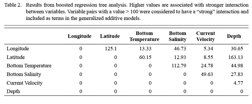
Table 2
Model fitting and variable selection using BSP went through two iterations of term removal. Depth was removed during the first round and bottom temperature was removed during the second round. Deviance explained for the parsimonious BSP model was 48.60 %. Model fitting and variable selection using TPRS, similarly, penalized depth to a high degree (edf = 0.05, Table 3, Fig. 4) to where it had a negligible effect on predictions. The effect of both bottom temperature (edf = 0.91) and longitude (edf = 0.94) on scallop density were reduced to almost linear relationships (Table 3, Fig. 4). Deviance explained for the parsimonious TPRS model was 49.70% (Table 3).
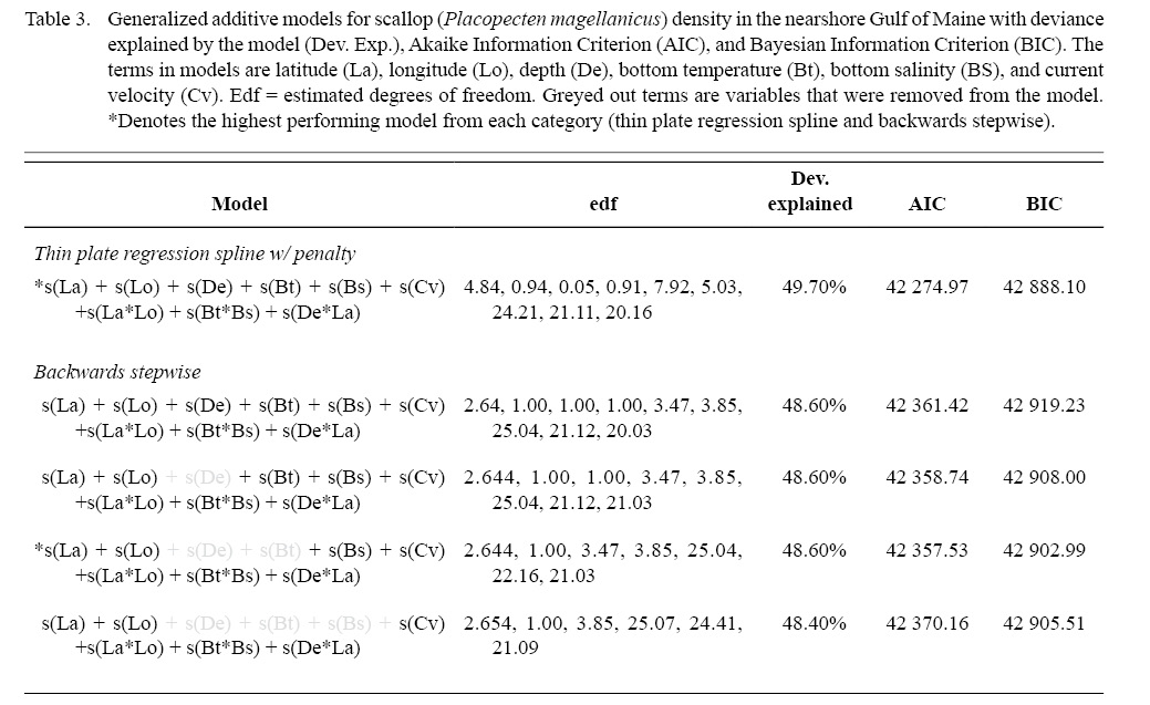
Table 3
While overall model performance was similar between the parsimonious BSP and TPRS GAMs, TPRS model slightly outperformed BSP model across all evaluation criteria (Table 3, Fig. 6). AIC and BIC were lower in the TPRS model (AIC = 42 274.97, BIC = 42 888.10), suggesting its superior performance over the BSP model (Table 3). Assessed by cross validation, the TPRS model showed higher predictive performance (α = -0.60, β = 1.02, R2 = 0.42) compared to the BSP model (α = -2.278, β = 1.04, R2 = 0.41; Fig. 6). Therefore, the TPRS model was determined to be more appropriate than the BSP model in this study.
Model predictions.
The parsimonious TPRS GAM was used to map model predictions over the inshore GoM. Model results show that nonlinear relationships commonly exist between environmental variables and scallop density; however, both bottom temperature and longitude were reduced to decreasing, near-linear relationships by the TPRS model. The response curves for scallop density as a function of bottom salinity and current velocity were dome shaped, with salinity peaking between 27–32 ppt and current velocity peaking between 0.10–0.17 (m/s). Because depth was penalized out of the TPRS model, this response curve was flat.
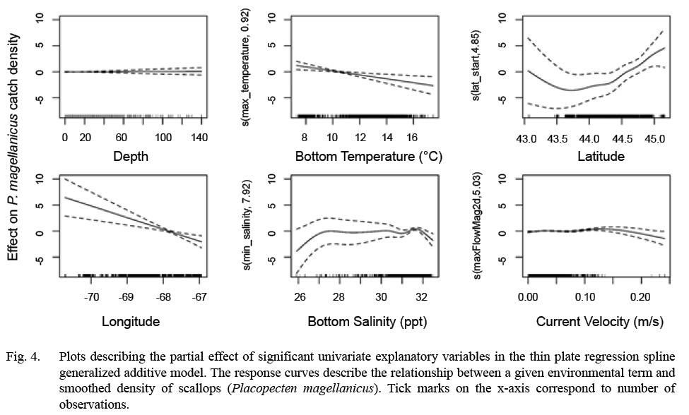
Fig. 4
Interactions included in this model (latitude-longitude, latitude-depth, bottom temperature-bottom salinity), identified using BRT analysis, were included to capture the common effect of single environmental variables operating within a more complex composite of factors directly controlling species distribution (Austin, 2007, Araujo and Peterson, 2012). For example, salinity in this model acts as a proxy for broad spatial patterns in scallop distribution which is shown by the strong interaction between salinity and temperature detected within the model, and likely corresponds to the origin of water mass existing in a given area (MacDonald and Thompson, 1985a, 1985b; Macdonald et al., 1987).
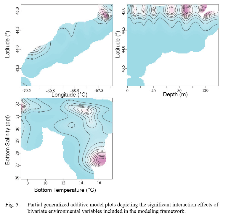
Fig. 5
Predicted scallop density was higher (>20 scallops per m2), in general, along inshore areas relative to offshore areas (<5 scallops per m2) (Fig. 7). Select estuaries along the Maine coast show significantly higher (>60 scallops per m2) predicted scallop density relative to other inshore areas. In particular, the Cobscook Bay area shows high predicted density (>100 scallops per m2) relative to surrounding areas (Fig. 7). Additionally, offshore waters in Western Maine show slightly higher predicted density (10–20 scallops per m2) relative to Eastern Maine (<10 scallops per m2) (Fig. 7). Over the 8-year study, predicted density shows a strong increasing trend along inshore areas and a decreasing trend in offshore areas (Fig. 8). Cobscook Bay and Penobscot Bay show stronger increasing trends relative to other inshore areas and offshore waters in Western Maine show a stronger decreasing trend in predicted density relative to Eastern Maine.
Discussion
Decision-making associated with conservation planning and fisheries management should use as much information and knowledge as possible to maximize the benefits of management actions (De Ornellas et al., 2011). The model developed in our study was designed to use an existing dataset describing both the abundance and distribution of Atlantic sea scallops to develop a climate-niche species distribution model (SDM). Our Tweedie GAM approach produced high quality predictions of abundance for scallops. Model outputs agree generally with consensus of the distribution of scallops along coastal Maine according to fishermen knowledge, the distribution of fishing effort in the area, as well as landings information (not able to be shown here due to confidentiality agreements). Thus, we consider this modeling effort a successful approach to predict the distribution of scallops across unsampled areas.
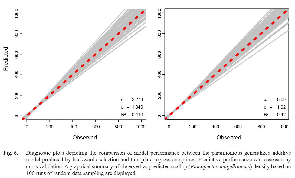
Fig. 6
This study provides a regional projection in the distribution of scallops within the inshore GoM and hindcasts these projections back eight years. A dominant spatial trend made apparent by this climate-niche SDM is a decline in predicted density moving from inshore to offshore locations. This finding corresponds with habitat value for scallops being higher among inshore areas relative to offshore areas likely attributed to deteriorating food availability moving offshore (Torre et al., 2018). This is thought to represent a natural gradient of habitat quality (Sarro and Stokesbury, 2009).
An increasing temporal trend in climate-driven scallop density was observed for inshore areas with a decreasing trend in offshore areas (Fig. 8). Any change in density over time results from changes in dynamic environmental variables (bottom temperature, bottom salinity, and current velocity), suggesting that the composite of these three factors has changed favorably regarding scallop abundance from 2005–2013 in inshore areas and has changed unfavorably in offshore areas. These trends assume that scallop-environment relationships have remained consistent over the study period (Pearson and Dawson, 2003, Crisp et al., 2009, Catullo et al., 2015). This general temporal trend is reflected in a recent study which depicts the spatiotemporal distribution of available scallop habitat in the GoM using a bioclimate envelope model (Torre et al., 2018).
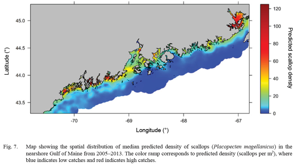
Fig. 7
The TPRS GAM, incorporating a Tweedie distribution for zero-inflated catch data was shown to be a useful prediction tool according to cross validation. The response curves in general agreed with known information about drivers of scallop distribution (Naidu and Anderson, 1984; Thouzeau et al., 1991; Wildish and Kristmason, 1993; Stewart and Arnold, 1994; Pilditch and Grant, 1999; Hart and Chute, 2004; Torre et al., 2018).
Depth in the case of this modeling framework was not significant, and so was penalized out of the TPRS model. In other studies, scallops have been shown to grow more slowly (MacDonald and Thompson, 1985; Thouzeau et al., 1991) and occur at reduced densities (Schick et al., 1988; Shumway and Parsons, 2006) at deeper depths; however, the example given here is comprised of areas that were surveyed in less than 100 m, as opposed to scallops occupying deep areas in other studies (up to 170 m in the case of Schick et al., 1988). Since, within the current study, the dataset describing scallop distribution has low contrast in depth, it follows that depth is not a critical environmental component in this modeling framework.
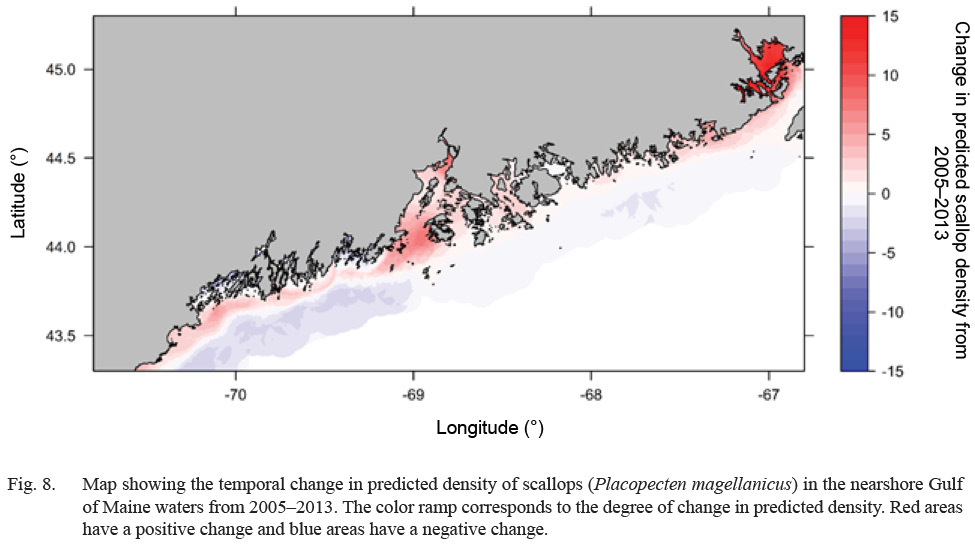
Fig. 8
The results show that, overall, a shrinkage approach where each variable in the full GAM was fitted with a thin plate regression spline including a thin plate spline penalty (TPRS) performed better across all model evaluation criteria than a classic, backwards selection procedure (BSP) for predicting scallop density. These results support findings from Marra and Wood (2011), which used simulated data to show that shrinkage approaches perform significantly better than competing approaches (including BSP) in terms of predictive ability, and are competitive in terms of variable selection performance. However, when using simulated data, the advantage of one modeling approach over another depends on the underlying structure of the simulated data, which makes it difficult to select a “best procedure” for all situations (Binder and Tutz, 2008). For example, Marra and Wood (2011) suggest that BSP would be preferred over shrinkage approaches in situations where the data have particularly high information content. Hence, using real-world data to evaluate the utility of model fitting and variable selection methods, as they apply to species distribution modeling, adds an important dimension to comparisons made with simulated data.
In addition to direct model performance benefits offered by TPRS, compared to BSP, shown here and in Marra and Wood (2011), there are other considerations that need to be taken into account when choosing an appropriate method for model fitting and variable selection. Stepwise procedures, such as BSP, have the potential to be inconsistent due to high sensitivity to small variability in the response data, which can sometimes lead to very different subsets of chosen variables. Additional variation in application of stepwise procedures results from a dependence on the initial starting path chosen through the variable space (Marra and Wood, 2011). Another downside of these procedures is that during variable selection and hypothesis testing using the selected model, p-values associated with model terms do not take into account variable selection uncertainty, and can therefore be misleading (Marra and Wood, 2011). Conversely, shrinkage approaches have been shown to be a valid alternative to stepwise procedures in terms of consistency among iterations of application, and increased robustness to variability in the data (Marra and Wood, 2011). Moreover, since variable selection in shrinkage approaches is carried out within a single step these methods are less computationally demanding, especially when using larger datasets (Leathwick et al., 2006, Hesterberg et al., 2008).
An important limitation of this modeling framework is that the development of species distribution models relies upon environmental data, and as with any environmental data there are several possible sources of error that could cause misrepresentation of model predictions. The current modeling framework relies particularly heavily upon FVCOM predictions. To evaluate performance of FVCOM within the study area, Tanaka and Chen (2016) and Li et al., (2017) performed comparisons between environmental monitors on observed temperature data to and FVCOM predictions. They found that in general, FVCOM adequately captured broad spatial and temporal trends in bottom temperature and salinity which adds validity to the quality and accuracy of FVCOM predictions.
In this study, environment-density relationships for scallops were defined upon only four environmental variables when, many physical, biological, and chemical conditions likely factor into the life history and distribution of this species. However, variables used to train the generalized additive model may have functioned as surrogates for factors directly controlling scallop distribution through physiological mechanisms (Austin, 2007; Araujo and Peterson, 2012). From the associations between variables we can infer the relationship between spatiotemporal variability of environmental factors, habitat quality, and resulting scallop distribution. For example, salinity in this model may act as a proxy for broad scale spatial patterns in scallop distribution due to the inherent relationship between salinity and the origin of water mass existing in a given area. Environmental predictors in this study were selected based on availability and assumed correlation with scallop density. As more comprehensive environmental data becomes available in the future, studies to develop a further detailed species distribution modeling approach could include additional variables such as pH, dissolved oxygen, predator-prey, and other food-web interactions to capture a more comprehensive representation of scallop ecology (Araújo and Luoto, 2007).
The climate-niche SDM developed in this study establishes the ability to quantify relationships between a commercially important fish stock and the surrounding environment, which provides a tangible tool to visualize species distribution over space and time as well as to evaluate potential impacts of a changing GoM ecosystem. Also, our real-world evaluation of two common GAM selection and fitting procedures provides insights into the effectiveness of each method and can be incorporated into further research using GAMs. This modeling approach is highly generalizable to a variety of commercially important species and can advise conservation efforts for the scallop fishery in the GoM to help ensure the implementation of adaptive management strategies under uncertain climate conditions.
Acknowledgements.
We thank Kevin Kelly and Mike Kersula of Maine Department of Marine Resources for providing survey and interview data along with model feedback. This research was supported by the US National Science Foundation Adaptation to Abrupt Climate Change IGERT program grant DGE-1144423, NOAA Scallop RSA fund, NSF Coastal SEES program and Maine Sea Grant College Program. This work uses the FVCOM developed by Dr. Changsheng Chen’s research team at the Marine Ecosystem Dynamics Modeling Laboratory, University of Massachusetts Dartmouth.
References
Akaike, H. (1974). A new look at the statistical model identification. Trans. Autom. Contr., 19: 716–723. https://doi.org/10.1109/TAC.1974.1100705.
Araújo, M. B., and Luoto, M. (2007). The importance of biotic interactions for modelling species distributions under climate change. Glob. Ecol. Biogeogr., 16: 743–753
https://doi.org/10.1111/j.1466-8238.2007.00359.x.
Araujo, M. B., and Peterson, A. T. (2012). Uses and misuses of bioclimatic envelope modeling. Ecology, 93: 1527–1539
https://doi.org/10.1890/11-1930.1.
Austin, M. (2007). Species distribution models and ecological theory: A critical assessment and some possible new approaches. Ecol. Modell., 200: 1–19
https://doi.org/10.1016/j.ecolmodel.2006.07.005.
Bailey, T. C., and Gatrell A. C. (1995). Interactive spatial data analysis. Longman Scientific and Technical.
Binder, H., and Tutz, G. (2008). A comparison of methods for the fitting of generalized additive models. Stat. Comput., 18: 87–99. https://doi.org/10.1007/s11222-007-9040-0
Boulangeat, I., Gravel, D., and Thuiller, W. (2012). Accounting for dispersal and biotic interactions to disentangle the drivers of species distributions and their abundances. Ecol. Lett., 15: 584–593. https://doi.org/10.1111/j.1461-0248.2012.01772.x.
Burnham, K. P., and Anderson, D. R. (2002). Model selection and multimodel inference. Springer Science + Business Media, New York.
Caddy, J. (1979). Long-term trends and evidence for production cycles in the Bay of Fundy scallop fishery. Rappel. Proces-Verbaux des Reun. Conscil Int. pour l’Exploration la Mer 15: 97–108.
Carsen, A. E., Hatcher, B.G., Scheibling, R. E., Hennigar, A. W, and Taylor, L. H. (1995). Effects of site and season on movement frequencies and displacement patterns of juvenile sea scallops Placopecten magellanicus under natural hydrodynamic conditions in Nova Scotia, Canada. Mar. Ecol. Prog. Ser., 128: 225–238. https://doi.org/10.3354/meps128225.
Catullo, R. A., Ferrier, S., and Hoffmann, A. A. (2015). Extending spatial modelling of climate change responses beyond the realized niche: Estimating, and accommodating, physiological limits and adaptive evolution. Glob. Ecol. Biogeogr. 24: 1192–1202. https://doi.org/10.1111/geb.12344.
Chen, C., Beardsley, R. C., and Cowles, G. (2006). An unstructured-grid, finite-volume coastal ocean model (FVCOM) system. Oceanography, 19: 78–89. https://doi.org/10.5670/oceanog.2006.92.
Chen, C., Beardsley, R., Cowles, G., Qi, J., Lai, Z., Gao, G., Stuebe, D., Xu, Q., Xue, P., Ge, J., Ji, R., Hu, S., Tian, R., Huang, H., Wu, L., and Lin, H. (2011). An unstructured-grid, finite-volume community ocean model fvcom user manual. 3rd edition.
Crisp, M. D., Arroyo, M.T. K., Cook, L. G., Gandolfo, M. A., Jordan, G. J., McGlone, M. S., Weston, P. H., Westoby, M., Wilf, P., and Linder, H. P. (2009). Phylogenetic biome conservatism on a global scale. Nature, 458: 754–756. https://doi.org/10.1038/nature07764.
Dickie, L. (1955). Fluctuations in abundance of the giant scallop, Placopecten magellanicus (Gmelin), in the Digby area of the Bay of Fundy. J. Fish. Res. Board Canada, 12: 797–857
https://doi.org/10.1139/f55-045.
Drinkwater, K. F., and Gilbert, D. (2004). Hydrographic variability in the waters of the Gulf of St. Lawrence, the Scotian Shelf and the eastern Gulf of Maine (NAFO Subarea 4) during 1991–2000. J. Northwest Atl. Fish. Sci., 34: 85–101. https://doi.org/10.2960/J.v34.m545.
Elith, J., Leathwick, J.R., and Hastie, T. (2008). A working guide to boosted regression trees. J. Anim. Ecol., 77: 802–813.
https://doi.org/10.1111/j.1365-2656.2008.01390.x.
Frank, K. T., Perry, R. I., and Drinkwater, K. F. (1990). Predicted Response of Northwest Atlantic Invertebrate and Fish Stocks to CO2-Induced Climate Change. Trans. Am. Fish. Soc., 119: 335–365. https://doi.org/10.1577/1548-8659(1990)119%3C0353:PRONAI%3E2.3.CO;2.
Franklin, J. (2010). Mapping Species Distributions. Spatial Inference and Prediction. Cambridge University Press
https://doi.org/10.1017/CBO9780511810602.
Guisan, A., Edwards, T.C., and Hastie, T. (2002). Generalized linear and generalized additive models in studies of species distributions: setting the scene. Ecol. Modell. 157: 89–100
https://doi.org/10.1016/S0304-3800(02)00204-1.
Hart D. R., and Chute A. S. (2004). Essential Fish Habiat Source Document: Sea Scallop, Placopecten magellanicus, Life History and Habitat Characteristics.
Hastie, T. (2009). The elements of statistical learning: data mining, inference, and prediction. Springer.
Hesterberg,T., Choi, N. H., Meier, L., and Fraley, C. (2008). Least angle and penalized regression: A review. Stat. Surv. 2: 61–93. https://doi.org/10.1214/08-SS035.
Hijmans, R. J., Philips, S., Leathwick, J. R., and Elith, J. (2017). dismo: Species Distribution Modeling. https://cran.r-project.org/web/packages/dismo/ (accessed02.04.13).
Hollowed, A. B., Planque, B., and Loeng, H. (2013). Potential movement of fish and shellfish stocks from the sub-Arctic to the Arctic Ocean. Fish. Oceanogr. 22: 355–370.
https://doi.org/10.1111/fog.12027.
Howell, P., and Auster, P.J. (2012). Phase Shift in an Estuarine Finfish Community Associated with Warming Temperatures. Mar. Coast. Fish., 4: 481–495. https://doi.org/10.1080/19425120.2012.685144.
Kelly, K. H. (2012). Results from the 2011 Maine sea scallop survey.
Kurihara, H. (2008). Effects of CO2-driven ocean acidification on the early developmental stages of invertebrates. Mar. Ecol. Prog. Ser. 373: 275–284. https://doi.org/10.3354/meps07802.
Leathwick, J. R., Elith J., and Hastie, T. (2006). Comparative performance of generalized additive models and multivariate adaptive regression splines for statistical modelling of species distributions. Ecol. Modell. 199: 188–196.
https://doi.org/10.1016/j.ecolmodel.2006.05.022.
Li, Y., Jiao, Y., and He, Q. (2011). Decreasing uncertainty in catch rate analyses using Delta-AdaBoost: An alternative approach in catch and bycatch analyses with high percentage of zeros. Fish. Res., 107: 261–271. https://doi.org/10.1016/j.fishres.2010.11.008.
Li, B., Tanaka, K.R., Chen, Y., Brady, D.C., and Thomas, A. C. (2017). Assessing the quality of bottom water temperatures from the Finite-Volume Community Ocean Model (FVCOM) in the Northwest Atlantic Shelf region. J. Mar. Syst. 173: 21–30. https://doi.org/10.1016/j.jmarsys.2017.04.001.
MacDonald, B., and Thompson, R. (1985). Influence of temperature and food availability on the ecological energetics of the giant scallop Placopecten magellanicus. II. Reproductive output and total production. Mar. Ecol. Prog. Ser., 25: 295–303. https://doi.org/10.3354/meps025279. https://doi.org/10.3354/meps025295.
Marra G., and Wood S.N. (2011). Practical variable selection for generalized additive models. Comput. Stat. Data Anal. 55: 2372–2387. https://doi.org/10.1016/j.csda.2011.02.004
Mendo T., Lyle J. M., Moltschaniwskyj N. A., Tracey S. R., Semmens J.M. (2014). Habitat characteristics predicting distribution and abundance patterns of scallops in D’Entrecasteaux Channel, Tasmania. PLoS One, 9: 1–9. https://doi.org/10.1371/journal.pone.0085895.
Merow C., Smith M. J., Edwards T. C., Guisan A., Mcmahon S.M., Normand S., Thuiller W., Wüest R. O., Zimmermann N.E., and Elith J. (2014). What do we gain from simplicity versus complexity in species distribution models? Ecography, (Cop) 37:1267–1281. https://doi.org/10.1111/ecog.00845.
Mills K. E., Pershing A. J., Brown C. J., Chen Y., Chiang F.-S., Holland D. S., Lehuta S., Nye J. A., Sun J. C., Thomas A. C., and Wahle R. A. (2013). Fisheries management in a changing climate: Lessons from the 2012 ocean heat wave in the northwest Atlantic. Oceanography, 26: 191–195. https://doi.org/10.5670/oceanog.2013.27.
Naidu K., and Anderson J. (1984). Aspects of scallop recruitment on St. Pierre Bank in relation to oceanography and implications for resource management. Can. Atl. Fish. Sci. Adv. Comm. Res. Doc. 84: 9 p.
National Geophysical Data Center. (1999). U.S. Coastal Relief Model - Northeast Atlantic.
Nye J. A., Link J. S., Hare J. A., and Overholtz W. J. (2009). Changing spatial distribution of fish stocks in relation to climate and population size on the Northeast United States continental shelf. Mar. Ecol. Prog. Ser., 393: 111–129
https://doi.org/10.3354/meps08220.
Ornellas P. De, Milner-Gulland E. J., Nicholson E. (2011). The impact of data realities on conservation planning. Biol. Conserv., 144: 1980–1988. https://doi.org/10.1016/j.biocon.2011.04.018.
Overholtz W. J., Hare J. A., and Keith C. M. (2011). Impacts of Interannual Environmental Forcing and Climate Change on the Distribution of Atlantic Mackerel on the U.S. Northeast Continental Shelf. Mar. Coast Fish. 3: 219–232.
https://doi.org/10.1080/19425120.2011.578485
Pearson R. G., Dawson T. P. (2003). Predicting the impacts of climate change on the distribution of species : are bioclimate envelope models useful? Glob. Ecol. Biogeogr. 12: 361–371. https://doi.org/10.1046/j.1466-822X.2003.00042.x.
Pershing A. J., Alexander M. A., Hernandez C. M., Kerr L. A., Bris A. Le, Mills K. E., Nye J. A., Record N. R. , Scannell H. A., Scott J. D., Sherwood G. D., and Thomas A. C. (2015). Slow adaptation in the face of rapid warming leads to collapse of the Gulf of Maine cod fishery. Science (80- ) 350: 809–812. https://doi.org/10.1126/science.aac9819.
Pilditch C. A., and Grant J. (1999). Effects of variation in flow velocity and phytoplankton concentration on sea scallop (Placopecten magellanicus) grazing rates. J. Exp. Mar. Bio. Ecol., 240: 111–136. https://doi.org/10.1016/S0022-0981(99)00052-0.
R Core Development Team. (2016) R: A language and environment for statistical computing.
Sagarese S. R., Frisk M. G., Cerrato R. M., Sosebee K. A., Musick J. A. , and Rago P. J. (2014). Application of generalized additive models to examine ontogenetic and seasonal distributions of spiny dogfish (Squalus acanthias) in the Northeast (US) shelf large marine ecosystem. Can. J. Fish. Aquat. Sci., 71: 847–877. https://doi.org/10.1139/cjfas-2013-0342.
Sarro C. L., and Stokesbury K. D. E. (2009). Spatial and temporal variation in the shell height/meat weight relationship of the sea scallop Placopecten magellanicus in the Georges Bank fishery. J. Shellfish Res. 28: 497–503. https://doi.org/10.2983/035.028.0311.
Schick D., Shumway S., and Hunter M. (1988). A comparison of growth rate between shallow water and deep water populations of scallops, Placopecten magellanicus(Gmelin, 1791), in the Gulf of Maine. Am. Malacol. Bull. 6: 1–8.
Shono H. (2008) Application of the Tweedie distribution to zero-catch data in CPUE analysis. Fish Res. 93: 154–162.
https://doi.org/10.1016/j.fishres.2008.03.006.
Shumway S. E., Parsons G. J. (2006). Scallops: Biology, Ecology and Aquaculture. Elsevier
Smith P. A. (1994). Autocorrelation in Logistic Regression Modelling of Species’ Distributions. Glob. Ecol. Biogeogr. Lett., 4: 47–61. https://doi.org/10.2307/2997753
Stewart P., and Arnold S. (1994). Environmental requirements of the sea scallop (Placopecten magellanicus) in eastern Canada and its response to human impacts. Can. Tech. Rep. Fish. Aquat. Sci. 2005: 1–36
Stokesbury K. D. E., and Himmelman J. H. (1995) Biological and physical variables associated with aggregations of the giant scallop Placopecten magellanicus. Can. J. Fish. Aquat. Sci., 52:743–753. https://doi.org/10.1139/f95-074.
Tanaka K. R., Chang J.-H., Xue Y., Li Z., Jacobson L., and Chen Y. (2018). Mesoscale climatic impacts on the distribution of Homarus americanus in the US inshore Gulf of Maine. Can. J. Fish. Aquat. Sci., 76(4): 608–625. https://doi.org/10.1139/cjfas-2018-0075.
Tanaka K., and Chen Y. (2015). Spatiotemporal variability of suitable habitat for American lobster (Homarus Americanus) in Long Island Sound. J. Shellfish Res., 34: 531–543. https://doi.org/10.2983/035.034.0238.
(2016) Modeling spatiotemporal variability of the bioclimate envelope of Homarus americanus in the coastal waters of Maine and New Hampshire. Fish. Res., 177: 137–152. https://doi.org/10.1016/j.fishres.2016.01.010.
Thouzeau G., Robert G., and Smith S. J. (1991). Spatial variability in distribution and growth of juvenile and adult sea scallops Placopecten magellanicus (Gmelin) on eastern Georges Bank (northwest Atlantic). Mar. Ecol. Prog. Ser., 74: 205–218. https://doi.org/10.3354/meps074205.
Torre M. P., Tanaka K. R., and Chen Y. (2018). A spatiotemporal evaluation of Atlantic sea scallop Placopecten magellanicus habitat in the Gulf of Maine using a Bioclimate Envelope Model. Mar. Coast. Fish. 10: 224–235.
https://doi.org/10.1002/mcf2.10022
Tremblay, M. J. (1997) Snow crab (Chionoecetes opilio) distribution limits and abundance trends on the Scotia Shelf. J. Northw. Atl. Fish. Sci., 21: 7–21.
https://doi.org/10.2960/J.v21.a1
Wildish, D., and Kristmason, D. (1993). Bivalve Filter Feeders in Estuarine and Coastal Ecosystem Processes. In: NATO ASI Series.
Wildish, D. J., and Saulnier, A. M. (1992). The effect of velocity and flow direction on the growth of juvenile and adult giant scallops. J. Exp. Mar. Bio. Ecol., 133: 133–143.
https://doi.org/10.1016/0022-0981(92)90032-6
Wood, S. N. (2003). Thin plate regression splines. J. R. Stat. Soc. B., 65: 95–114. https://doi.org/10.1111/1467-9868.00374
(2006) Generalized additive models: an introduction with R. Chapman and Hall, London. https://doi.org/10.1201/9781420010404
(2011). Fast stable REML and ML estimation of semiparametric GLMs. J. R. Stat. Soc. Ser B. (Statistical Methodol., 73: 3–36. https://doi.org/10.1111/j.1467-9868.2010.00749.x
Young, M., and Carr, M. H. (2015). Application of species distribution models to explain and predict the distribution, abundance and assemblage structure of nearshore temperate reef fishes. Divers. Distrib. 21: 1428–1440.
https://doi.org/10.1111/ddi.12378
Zuur, A. F., Ieno, E. N., and Smith, G. M. (2007). Analysing Ecological Data. Springer Science and Business Media.
https://doi.org/10.1007/978-0-387-45972-1
Zuur, A. F., Ieno, E. N., Walker, N. J., Saveliev, A. A., and Smith, G. M. (2009). Mixed effects models and extensions in ecology with R. Springer, New York.
https://doi.org/10.1007/978-0-387-87458-6
Citation: Torre, M.P., K.R. Tanaka, and Y. Chen. 2019. Development of a climate-niche model to evaluate spatiotemporal trends in
Placopecten magellanicus distribution in the Gulf of Maine, USA.
J. Northw. Atl. Fish. Sci.,
50: 37–50. https://doi.org/10.2960/J.v50.m721